AD Forward Mode - Advanced Use in MATLAB

5 Advanced Use of Forward Mode for First Derivatives

We have seen in section 4 how Mad via overloaded operations on variables of the fmad class may calculate first derivatives. In this section we explore more advanced use of the fmad class.

5.1 Accessing The Internal Representation of Derivatives

We saw in section 4 that fmad returns multiple derivatives as N-D arrays of one dimension higher than the corresponding value. Since Matlab variables are by default matrices, i.e. arrays of dimension 2, then we see that by default for multiple directional derivatives fmad will return 3-D (or higher dimension arrays). Although this approach is systematic it can be inconvenient. Frequently we require the Jacobian matrix of a vector valued function. We can trivially reshape or squeeze the 3-D array obtained by fmad to get the required matrix. However, and as we shall see in Section 5.3, this approach will not work if we wish to use Matlab's sparse matrix class to propagate derivatives. We should bear in mind that the derivvec class stores arbitrary dimension derivative arrays internally as matrices. This internal representation of the derivatives may be accessed directly through use of the function getinternalderivs as the following example shows.

Example 1

MADEXIntRep1: Internal Representation

This example illustrates MAD's internal representation of derivatives.

See also fmad, MADEXExtRep1, MADEXExtRep2

Contents

Define a vector [1;1] with derivatives given by the sparse identity
Getderivs returns the external form in full storage
Getinternalderivs returns the internal form

Define a vector [1;1] with derivatives given by the sparse identity


format compact
a=fmad([1;1],speye(2))

value =
     1
     1
Derivatives
Size = 2  1
No. of derivs = 2
d =
   (1,1)        1
d =
   (2,1)        1

Getderivs returns the external form in full storage


da=getderivs(a)

da(:,:,1) =
     1
     0
da(:,:,2) =
     0
     1

Getinternalderivs returns the internal form

getinternalderivs maintains the sparse storage used internally by MAD's derivvec class.


da=getinternalderivs(a)

da =
   (1,1)        1
   (2,2)        1

See Section 5.3 for more information on this topic.

5.2 Preallocation of Matrices/Arrays

It is well-known in Matlab that a major performance overhead is incurred if an array is frequently increased in size, or grown, to accommodate new data as the following example shows.

Example 2

MADEXPrealloc1: importance of array preallocation

This example illustrates the importance of preallocation of arrays when using MAD.

Contents

Simple loop without preallocation
Simple loop with preallocation
Fmad loop without preallocation
Fmad loop with preallocation

Simple loop without preallocation

Because the array a continuously grows, the following loop executes slowly.


format compact
clear a
n=5000;
x=1;
a(1)=x;
tic; for i=1:n; a(i+1)=-a(i);end; t_noprealloc=toc

t_noprealloc =
    0.0563

Simple loop with preallocation

To improve performance we preallocate a.


clear a
a=zeros(n,1);
a(1)=x;
tic; for i=1:n;a(i+1)=-a(i);end;t_prealloc=toc

t_prealloc =
    0.0089

Fmad loop without preallocation

With an fmad variable performance is even more dramatically reduced when growing an array.


clear a
x=fmad(1,[1 2]);
a(1)=x;
tic;for i=1:n;a(i+1)=-a(i);end;t_fmadnoprealloc=toc

t_fmadnoprealloc =
   15.1634

Fmad loop with preallocation

To improve performance we preallocate a.


clear a
a=zeros(n,length(x));
a(1)=x;
tic; for i=1:n;a(i+1)=-a(i);end;t_fmadprealloc=toc

t_fmadprealloc =
    4.5518

Note that we have preallocated a using zeros(n,length(x)). In fmad we provide fucntions length, size and numel that return, instead of the expected integers, fmad object results with zero derivatives. This then allows for them to be used in functions such as zeros (here) or ones to preallocate fmad objects. Also note that it is not possible to change the class of the object that is being assigned to in Matlab so if we wish to assign fmad variables to part of an matrix/array then that array must already be preallocated to be of fmad class. This technique has previously been used by Verma [Ver98a, Ver98c] in his ADMAT package.

Example 3
In example 5 the input argument y to the function will be of fmad class. In the third non-comment line,


dydt = zeros(2*N,size(y,2));      % preallocate dy/dt

of the function of Figure 1 we see that size(y,2) is used as an argument to zeros to preallocate storage for the variable dydt. Since y is of class fmad then so will be the result of the size function, and hence so will be the result of the zeros function and hence dydt will be of class fmad. This will then allow for fmad variables to be assigned to it and derivatives will be correctly propagated.

We now see how to avoid problem 1 noted in Section 4.7.

Example 4
We make use of length, acting on an fmad variable to preallocate the array y to be of fmad class.


>> x=fmad(1,1);
>> y=zeros(2,length(x(1)));
>> y(1)=x;

5.3 Dynamic Propagation of Sparse Derivatives

Many practical problems either possess sparse Jacobians or are partially separable so that many intermediate expressions have sparse local Jacobians. In either case it is possible to take advantage of this structure when calculating F'(x) V in the cases when V is sparse. In particular using V=I_n, the identity matrix, facilitates calculation of the Jacobian F'(x). In order to do this we need to propagate the derivatives as sparse matrices. Matlab matrices (though not N-D arrays) may be stored in an intrinsic sparse format for efficient handling of sparse matrices [GMS91]. Verma's ADMAT tool [Ver98a] can use Matlab's sparse matrices to calculate Jacobians of functions which are defined only by scalars and vectors. In fmad careful design [For06] of the derivvec class for storage of derivatives has allowed us to propagate sparse derivatives for variables of arbitrary dimension (N-D arrays). In this respect fmad has a similar capability to the Fortran 90 overloading package ADO1 [PR98], and the Fortran source-text translation tool ADIFOR [BCH+98] which may make use of the SparseLinC library to form linear combinations of derivative vectors. See [Gri00, Chap. 6] for a review of this AD topic.

5.3.1 Use of Sparse Derivatives

In order to use sparse derivatives we initialise our independent variables with a sparse matrix. We use the feature of the fmad constructor (section 4.3) that the derivatives supplied must be of the correct number of elements and in column major order to avoid having to supply the derivative as an N-D array. As the following example shows, getinternalderivs must be used to access derivatives in their sparse storage format.

Example 5

Sparse1: Dynamic sparsity for Jacobians with fmad

This example illustrates use of dynamic sparsity when calculating Jacobians with fmad.

Contents

A function with sparse Jacobian
Initialising sparse derivatives
Using sparse derivatives
Extracting the derivatives
Accessing the internal derivative storage

A function with sparse Jacobian

As a simple, small example we take,

y = F(x_1, x_2)=[ x_1^2 + x_2
                     x_2^2   ]

for which

DF/Dy = [ 2x_1  1
            0   2x_2]

and at (x_1,x_2)=(1,2)' we have,

DF/Dy = [ 2  1
          0  4]

Initialising sparse derivatives

We set the derivatives using the sparse identity matrix speye. Note that fmad's deriv component stores the derivatives as a derivvec object with sparse storage as indicated by the displaying of only non-zero entries.


x=fmad([1 2],speye(2))

value =
     1     2
Derivatives
Size = 1  2
No. of derivs = 2
d =
   (1,1)        1
d =
   (1,2)        1

Using sparse derivatives

We perform any calculations in the usual way - clearly y has sparse derivatives.


y=[x(1)^2+x(2); x(2)^2]

value =
     3
     4
Derivatives
Size = 2  1
No. of derivs = 2
d =
   (1,1)        2
d =
   (1,1)        1
   (2,1)        4

Extracting the derivatives

If we use getderivs then, as usual MAD insists on returning a 3_D array and sparsity information is lost.


dy=getderivs(y)
dy=reshape(dy,[2,2])

dy(:,:,1) =
     2
     0
dy(:,:,2) =
     1
     4
dy =
     2     1
     0     4

Accessing the internal derivative storage

By accessing the internal derivative storage used by fmad in its calculation, the sparse Jacobian can be extracted.


J=getinternalderivs(y)

J =
   (1,1)        2
   (1,2)        1
   (2,2)        4

The above example, though trivial, shows how sparse derivatives may be used in Mad. Of course there is an overhead associated with the use of sparse derivatives and the problem must be sufficiently large to warrant their use.

Example 6

MADEXbrussodeJacSparse: Brusselator Sparse Jacobian

This example shows how to use the fmad class to calculate the Jacobian of the Brusselator problem using sparse propagation of derivatives. The compressed approache of MADEXbrussodeJacComp may be more efficient.

See also: brussode_f, brussode_S, MADEXbrussodeJac, MADEXbrussodeJacComp, brussode

Contents

Initialise Variables
Use fmad with sparse storage to calculate the Jacobian
Using finite-differencing
Comparing the AD and FD Jacobian

Initialise Variables

We define the input variables.


N=3;
t=0;
y0=ones(2*N,1);

Use fmad with sparse storage to calculate the Jacobian

We initialise y with the value y0 and derivatives given by the sparse identity matrix of size equal to the length of y0. We may then evaluate the function and extract the value and Jacobian.


y=fmad(y0,speye(length(y0))); % Only significant change from MADEXbrussodeJac
F=brussode_f(t,y,N);
F_spfmad=getvalue(F); % grab value
JF_spfmad=getinternalderivs(F) % grab Jacobian

JF_spfmad =
   (1,1)      -2.6400
   (2,1)       1.0000
   (3,1)       0.3200
   (1,2)       1.0000
   (2,2)      -1.6400
   (4,2)       0.3200
   (1,3)       0.3200
   (3,3)      -2.6400
   (4,3)       1.0000
   (5,3)       0.3200
   (2,4)       0.3200
   (3,4)       1.0000
   (4,4)      -1.6400
   (6,4)       0.3200
   (3,5)       0.3200
   (5,5)      -2.6400
   (6,5)       1.0000
   (4,6)       0.3200
   (5,6)       1.0000
   (6,6)      -1.6400

Using finite-differencing


y=repmat(y0,[1 2*N+1]);
y(:,2:end)=y(:,2:end)+sqrt(eps)*eye(2*N);
F=brussode_f(t,y,N);
F_fd=F(:,1);
JF_fd=(F(:,2:end)-repmat(F_fd,[1 2*N]))./sqrt(eps)

JF_fd =
   -2.6400    1.0000    0.3200         0         0         0
    1.0000   -1.6400         0    0.3200         0         0
    0.3200         0   -2.6400    1.0000    0.3200         0
         0    0.3200    1.0000   -1.6400         0    0.3200
         0         0    0.3200         0   -2.6400    1.0000
         0         0         0    0.3200    1.0000   -1.6400

Comparing the AD and FD Jacobian

The function values computed are, of course, identical. The Jacobians disagree by about 1e-8, this is due to the truncation error of the finite-difference approximation.


disp(['Function values norm(F_fd-F_spfmad)  = ',num2str(norm(F_fd-F_spfmad,inf))])
disp(['Function Jacobian norm(JF_fd-JF_spfmad)= ',num2str(norm(JF_fd-JF_spfmad,inf))])

Function values norm(F_fd-F_spfmad)  = 0
Function Jacobian norm(JF_fd-JF_spfmad)= 2.861e-008

5.3.2 User Control of Sparse Derivative Propagation

Some AD tools, for example ADO1 [PR98], ADIFOR [BCH+98], allow for switching from sparse to full storage data structures for derivatives depending on the number of non-zeros in the derivative. There may be some user control provided for this. The sparse matrix implementation of Matlab [GMS91] generally does not convert from sparse to full matrix storage unless a binary operation of a sparse and full matrix is performed. For example a sparse-full multiplication results in a full matrix. In the derivvec arithmetic used by fmad we presently provide no facilities for switching from sparse to full storage once objects have been created. Since MAD version 1.2, the derivvec class is designed to ensure that once calculations start with sparse derivatives, they continue with sparse derivatives. Any behaviour other than this is a bug and should be reported.

5.4 Sparse Jacobians via Compression

It is well known [Gri00, Chap. 7] that, subject to a favourable sparsity pattern of the Jacobian, the number of directional derivatives that need to be determined in order to form all entries of the Jacobian may be greatly reduced. This technique, known as Jacobian (row) compression, is frequently used in finite-difference approximations of Jacobians [DS96, Sec. 11.2], [NW99, p169-173]. Finite-differencing allows Jacobian-vector products to be approximated and can be used to build up columns, or linear combinations of columns, of the Jacobian. Use of sparsity and appropriate coloring algorithms frequently enables many columns to be approximated from one approximated directional derivative. This technique is frequently referred to as sparse finite-differencing however we shall use the term compressed finite-differencing to avoid confusion with techniques using sparse storage. The forward mode of AD calculates Jacobian-vector products exactly and, using the same colouring techniques as in compressed finite-differencing, may therefore calculate many columns of the Jacobian exactly by propagating just one directional derivative. Thus row compression may also be used by the fmad class of Mad.

Coleman and Verma [CV96] and, independently, Hossain and Steihaug [HS98] showed that since reverse mode AD may calculate vector-Jacobian products it may be used to calculate linear combinations of rows of the Jacobian. This fact is frequently utilised in optimisation in which an objective function with single output has its gradient, or row Jacobian calculated by the propagation of a single adjoint. These authors showed that by utilising both forward and reverse AD, and specialised colouring algorithms they could efficiently calculate sparse Jacobians which could not be calculated by sparse finite-differences. Such techniques are not available in Mad.

For a given sparsity pattern the row compression calculation proceeds as follows:

Calculate a good coloring from the given sparsity pattern using MADcolor.
Construct an appropriate seed matrix to initialise derivatives using MADgetseed.
Calculate the compressed Jacobian by using fmad to propagate derivatives, initialised by the seed matrix, through the function calculation to yield a compressed Jacobian.
The compressed Jacobian is uncompressed using MADuncompressJac to yield the required sparse Jacobian.

We use the Brusselator example again to illustrate this.

Example 7

MADEXbrussodeJacComp: Brusselator Compressed Jacobian

This example shows how to use the fmad class to calculate the Jacobian of the Brusselator problem using compressed storage. If a good coloring can be found then this approach is usually more efficient than use of sparse or full storage as in MADEXbrussodeJac and MADEXbrussodeJacSparse.

See also: brussode_f, brussode_S, MADEXbrussodeJac, MADEXbrussodeJacSparse, brussode

Contents

Initialise variables
Obtain the sparsity pattern
Determine the coloring
Determine the seed matrix
Calculate the compressed Jacobian using fmad
Uncompress the Jacobian
Using finite-differencing
Comparing the AD and FD Jacobians
Using compressed finite-differencing
Comparing the AD and compressed FD Jacobians

Initialise variables

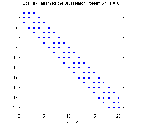
We define the input variables, setting N to 10 for this example.


format compact
N=10;
t=0;
y0=ones(2*N,1);

Obtain the sparsity pattern

The function brussode_S returns the sparsity pattern, the matrix with an entry 1 when the corresponding Jacobian entry is nonzero and entry 0 when the corresponding Jacobian entry is always zero.


sparsity_pattern=brussode_S(N);
figure(1)
spy(sparsity_pattern)
title(['Sparsity pattern for the Brusselator Problem with N=',num2str(N)])

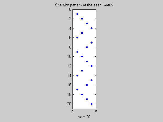
Determine the coloring

The function MADcolor takes the sparsity pattern and determines a color (or group number) for each component of the input variables so that perturbing one component with that color affects different dependent variables to those affected by any other variable in that group.


color_groups=MADcolor(sparsity_pattern);
ncolors=max(color_groups) % number of colors used

ncolors =
     4

Determine the seed matrix

The coloring is used by MADgetseed to determine a set of ncolors directions whose directional derivatives may be used to construct all Jacobian entries.


seed=MADgetseed(sparsity_pattern,color_groups);
figure(2);
spy(seed);
title('Sparsity pattern of the seed matrix')

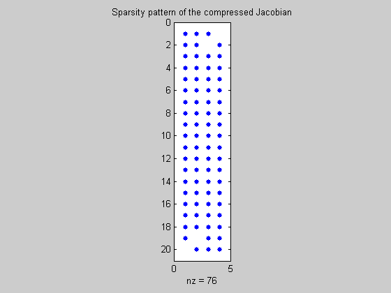
Calculate the compressed Jacobian using fmad

We initialise y with the value y0 and derivatives given by the seed matrix. We then evaluate the function and extract the value and compressed Jacobian.


y=fmad(y0,seed);
F=brussode_f(t,y,N);
F_compfmad=getvalue(F); % grab value
Jcomp=getinternalderivs(F); % grab compressed Jacobian
figure(3);
spy(Jcomp);
title('Sparsity pattern of the compressed Jacobian')

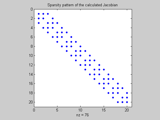
Uncompress the Jacobian

MADuncompressJac is used to extract the Jacobian from its compressed form.


JF_compfmad=MADuncompressJac(Jcomp,sparsity_pattern,color_groups);
figure(4);
spy(JF_compfmad);
title('Sparsity pattern of the calculated Jacobian')

Using finite-differencing


y=repmat(y0,[1 2*N+1]);
y(:,2:end)=y(:,2:end)+sqrt(eps)*eye(2*N);
F=brussode_f(t,y,N);
F_fd=F(:,1);
JF_fd=(F(:,2:end)-repmat(F_fd,[1 2*N]))./sqrt(eps);

Comparing the AD and FD Jacobians

The function values computed are, of course, identical. The Jacobians disagree by about 1e-8, this is due to the truncation error of the finite-difference approximation.


disp(['Function values norm(F_fd-F_compfmad)  = ',num2str(norm(F_fd-F_compfmad,inf))])
disp(['Function Jacobian norm(JF_fd-JF_compfmad)= ',num2str(norm(JF_fd-JF_compfmad,inf))])

Function values norm(F_fd-F_compfmad)  = 0
Function Jacobian norm(JF_fd-JF_compfmad)= 4.2915e-008

Using compressed finite-differencing

We may also use compression with finite-differencing.


y=repmat(y0,[1 ncolors+1]);
y(:,2:end)=y(:,2:end)+sqrt(eps)*seed;
F=brussode_f(t,y,N);
F_compfd=F(:,1);
Jcomp_fd=(F(:,2:end)-repmat(F_fd,[1 ncolors]))./sqrt(eps);
JF_compfd=MADuncompressJac(Jcomp_fd,sparsity_pattern,color_groups);

Comparing the AD and compressed FD Jacobians

The function values computed are, of course, identical. The Jacobians disagree by about 1e-8, this is due to the truncation error of the finite-difference approximation.


disp(['Function values norm(F_compfd-F_compfmad)  = ',num2str(norm(F_compfd-F_compfmad,inf))])
disp(['Function Jacobian norm(JF_compfd-JF_compfmad)= ',num2str(norm(JF_compfd-JF_compfmad,inf))])

Function values norm(F_compfd-F_compfmad)  = 0
Function Jacobian norm(JF_compfd-JF_compfmad)= 4.2915e-008

5.5 Differentiating Iteratively Defined Functions

Consider a function x → y defined implicitly as a solution of,

g(y,x)=0, (1)

and for which we require ∂ y/∂ x. Such systems are usually solved via some fixed point iteration of the form,

yⁿ⁺¹=h(yⁿ,x). (2)

There have been many publications regarding the most efficient way to automatically differentiate such a system [Azm97, BB98b, Chr94, Chr98] and reviewed in [Gri00]. A simple approach termed piggy-back [Gri00], is to use forward mode AD through the iterative process of equation 2. It is necessary to check for convergence of both the value and derivatives of y.

Example 8

MADEXBBEx3p1 - Bartholomew-Biggs Example 3.1 [BB98a]

This example demonstrates how to find the derivatives of a function defined by a fixed-point iteration using fmad. The example is taken from (M.C. Bartholomew-Biggs, "Using Forward Accumulation for Automatic Differentiation of Implicitly-Defined Functions", Computational Optimization and Applications 9, 65-84, 1998). The example concerns solution of

g₁=y₁−u₁+u₃*y₁*√

y₁²+y₂²

g₂=y₂−u₂+u₃*y₂*√

y₁²+y₂²

with

u₁=x₁*cos(x₂), u₂=x₁*sin(x₂), u₃=x₃

via the fixed-point iteration,

y_new=y_old−g(y_old).

5.6 User Control of Activities/Dependencies

Example 9 MADEXDepend1: User control of activities/dependencies

This example shows how a user may modify their code to render inactive selective variables which MAD automatically assumes are active.

See also: depend, depend2

Contents

Function depend
One independent variable
Dealing with one dependent variable

Function depend

The function depend defines two variables u,v in terms of independents x,y,

u=x+y, v=−x

Using the fmad class it is trivial to calculate the derivatives du/dx, du/dy, dv/dx, dv/dy. We associate the first directional derivative with the x-derivatives and the second with those of variable y.


format compact
x=fmad(1,[1 0]); y=fmad(2,[0 1]);
[u,v]=depend(x,y);
Du=getinternalderivs(u);
du_dx=Du(1)
du_dy=Du(2)
Dv=getinternalderivs(v);
dv_dx=Dv(1)
dv_dy=Dv(2)

du_dx =
     1
du_dy =
     1
dv_dx =
    -1
dv_dy =
     0

One independent variable

Dealing with one independent, say x, is trivial and here requires just one directional derivative.


x=fmad(1,1); y=2;
[u,v]=depend(x,y);
du_dx=getinternalderivs(u)
dv_dx=getinternalderivs(v)

du_dx =
     1
dv_dx =
    -1

Dealing with one dependent variable

When we are only interested in the derivatives of one dependent variable, say u, then things are more tricky since fmad automatically calculates derivatives of all variables that depend on active inputs. We could, of course, calculate v's derivatives and simply discard them and in many cases (including that here) the performance penalty paid would be insignificant. In some cases a calculation may be significant shortened by ensuring that we calculate derivatives only for those dependent variables we are interested in, or which are involved in calculating those dependents. To illustrate this see function depend2 in which we ensure v is not active by using MAD's getvalue function to ensure that only v's value and not its derivatives, is calculated. u=x+y; v=-getvalue(x); Note that in this case an empty matrix is returned by getinternalderivatives.


x=fmad(1,[1 0]); y=fmad(2,[0 1]);
[u,v]=depend2(x,y);
Du=getinternalderivs(u);
du_dx=Du(1)
du_dy=Du(2)
Dv=getinternalderivs(v)

du_dx =
     1
du_dy =
     1
Dv =
     []

The last case of just one active output is more difficult to deal with because derivatives are propagated automatically by fmad's overloaded library. Automatically dealing with a restricted number of active outputs requires a reverse dependency or activity analysis [Gri00]. This kind of analysis requires compiler based techniques and is implemented in source transformation AD tools such as ADIFOR, TAF/TAMCand Tapenade. In the present overloading context such an effect can only be achieved as above by the user carefully ensuring that unnecessary propagation of derivatives is stopped by judicious use of the getvalue function to propagate values and not derivatives. Of course such coding changes as those shown above, should only be performed if the programmer is sure they know what they are doing. Correctly excluding some derivative propagation and hence calculations may make for considerable run-time savings for large codes. However incorrect use will result in incorrectly calculated derivative values.

« Previous « Start » Next »