« Previous « Start » Next »
11 Batch Fermentor
Dynamic optimization of bioprocesses: efficient and robust numerical strategies 2003, Julio R. Banga, Eva Balsa-Cantro, Carmen G. Moles and Antonio A. Alonso
Case Study I: Optimal Control of a Fed-Batch Fermentor for Penicillin Production
11.1 Problem description
This problem considers a fed-batch reactor for the production of penicillin, as studied by Cuthrell and Biegler (1989). This problem has also been studied by many other authors (Dadebo & McAuley 1995, Banga & Seider 1996, Banga et al. 1997). We consider here the free terminal time version where the objective is to maximize the amount of penicillin using the feed rate as the control variable. It should be noted that the resulting NLP problem (after using CVP) does not seem to be multimodal, but it has been reported that local gradient methods do experience convergence problems if initialized with far-from-optimum profiles, or when a very refined solution is sought. Thus, this example will be excellent in order to illustrate the better robustness and efficiency of the alternative stochastic and hybrid approaches. The mathematical statement of the free terminal time problem is:
Find u(t) and t_f over t in [t0; t_f ] to maximize
subject to:
| h2 = 0.0055 * x3 * (0.0001 + x3*(1 + 10*x3)) |
where x1, x2, and x3 are the biomass, penicillin and substrate concentrations (g=L), and x4 is the volume (L). The initial conditions are:
There are several path constraints (upper and lower bounds) for state variables (case III of Cuthrell and Biegler, 1989):
The upper and lower bounds on the only control variable (feed rate of substrate) are:
Reference: [3]
11.2 Solving the problem on multiple grids.
The problem is solved in two stages. First, a solution is computed for a small number of collocation points, then the number of collocation points is increased, and the problem is resolved. This saves time, compared to using the fine grid immediately.
toms t
toms t_f

nvec = [35 70 80 90 100];

for i=1:length(nvec)
    n = nvec(i);
    p = tomPhase('p', t, 0, t_f, n);
    setPhase(p);

    tomStates x1 x2 x3 x4

    tomControls u

    % Initial guess
    % Note: The guess for t_f must appear in the list before
    % expression involving t.
    if i==1
        x0 = {t_f == 126
            icollocate(x1 == 1.5)
            icollocate(x2 == 0)
            icollocate(x3 == 0)
            icollocate(x4 == 7)
            collocate(u==11.25)};
    else
        % Copy the solution into the starting guess
        x0 = {t_f == tf_init
            icollocate(x1 == x1_init)
            icollocate(x2 == x2_init)
            icollocate(x3 == x3_init)
            icollocate(x4 == x4_init)
            collocate(u == u_init)};
    end

    % Box constraints
    % Setting the lower limit for t, x1 and x4 to slightly more than zero
    % ensures that division by zero is avoided during the optimization
    % process.
    cbox = {1 <= t_f  <= 256
        1e-8 <= mcollocate(x1) <= 40
        0    <= mcollocate(x2) <= 50
        0    <= mcollocate(x3) <= 25
        1    <= mcollocate(x4) <= 10
        0    <= collocate(u)   <= 50};

    % Various constants and expressions
    h1 = 0.11*(x3./(0.006*x1+x3));
    h2 = 0.0055*(x3./(0.0001+x3.*(1+10*x3)));

    % Boundary constraints
    cinit = initial({x1 == 1.5; x2 == 0
        x3 == 0; x4 == 7});

    % This final condition is not necesary, but helps convergence speed.
    cfinal = final(h2.*x1-0.01*x2) == 0;

    % ODEs and path constraints
    ceq = collocate({
        dot(x1) == h1.*x1-u.*(x1./500./x4)
        dot(x2) == h2.*x1-0.01*x2-u.*(x2./500./x4)
        dot(x3) == -h1.*x1/0.47-h2.*x1/1.2-x1.*...
        (0.029*x3./(0.0001+x3))+u./x4.*(1-x3/500)
        dot(x4) == u/500});

    % Objective
    objective = -final(x2)*final(x4);

    options = struct;
    options.name = 'Batch Fermentor';
    %options.scale = 'auto';
    %if i==1
    %    options.solver = 'multiMin';
    %    options.xInit = 20;
    %end
    solution = ezsolve(objective, {cbox, cinit, cfinal, ceq}, x0, options);
Problem type appears to be: qpcon
Starting numeric solver
===== * * * =================================================================== * * *
TOMLAB - Tomlab Optimization Inc. Development license  999001. Valid to 2011-02-05
=====================================================================================
Problem: ---  1: Batch Fermentor                f_k     -87.746072952335396000
                                       sum(|constr|)      0.000000000591461608
                              f(x_k) + sum(|constr|)    -87.746072951743940000
                                              f(x_0)      0.000000000000000000

Solver: snopt.  EXIT=0.  INFORM=1.
SNOPT 7.2-5 NLP code
Optimality conditions satisfied

FuncEv    1 ConstrEv  924 ConJacEv  924 Iter  275 MinorIter 4942
CPU time: 8.250000 sec. Elapsed time: 8.485000 sec.
Problem type appears to be: qpcon
Starting numeric solver
===== * * * =================================================================== * * *
TOMLAB - Tomlab Optimization Inc. Development license  999001. Valid to 2011-02-05
=====================================================================================
Problem: ---  1: Batch Fermentor                f_k     -87.965550967205928000
                                       sum(|constr|)      0.000000291694933232
                              f(x_k) + sum(|constr|)    -87.965550675510997000
                                              f(x_0)    -87.746072952334629000

Solver: snopt.  EXIT=0.  INFORM=1.
SNOPT 7.2-5 NLP code
Optimality conditions satisfied

FuncEv    1 ConstrEv   98 ConJacEv   98 Iter   58 MinorIter 1466
CPU time: 6.328125 sec. Elapsed time: 6.453000 sec.
Problem type appears to be: qpcon
Starting numeric solver
===== * * * =================================================================== * * *
TOMLAB - Tomlab Optimization Inc. Development license  999001. Valid to 2011-02-05
=====================================================================================
Problem: ---  1: Batch Fermentor                f_k     -87.989983108591034000
                                       sum(|constr|)      0.000000063125343100
                              f(x_k) + sum(|constr|)    -87.989983045465692000
                                              f(x_0)    -87.966078735435829000

Solver: snopt.  EXIT=0.  INFORM=1.
SNOPT 7.2-5 NLP code
Optimality conditions satisfied

FuncEv    1 ConstrEv  116 ConJacEv  116 Iter   92 MinorIter 2087
CPU time: 14.265625 sec. Elapsed time: 14.438000 sec.
Problem type appears to be: qpcon
Starting numeric solver
===== * * * =================================================================== * * *
TOMLAB - Tomlab Optimization Inc. Development license  999001. Valid to 2011-02-05
=====================================================================================
Problem: ---  1: Batch Fermentor                f_k     -88.030366209342986000
                                       sum(|constr|)      0.000000440801301912
                              f(x_k) + sum(|constr|)    -88.030365768541685000
                                              f(x_0)    -87.990147691715819000

Solver: snopt.  EXIT=0.  INFORM=1.
SNOPT 7.2-5 NLP code
Optimality conditions satisfied

FuncEv    1 ConstrEv   99 ConJacEv   99 Iter   88 MinorIter 1713
CPU time: 15.859375 sec. Elapsed time: 16.078000 sec.
Problem type appears to be: qpcon
Starting numeric solver
===== * * * =================================================================== * * *
TOMLAB - Tomlab Optimization Inc. Development license  999001. Valid to 2011-02-05
=====================================================================================
Problem: ---  1: Batch Fermentor                f_k     -88.044843218600391000
                                       sum(|constr|)      0.000000326396054727
                              f(x_k) + sum(|constr|)    -88.044842892204343000
                                              f(x_0)    -88.030366874603772000

Solver: snopt.  EXIT=0.  INFORM=1.
SNOPT 7.2-5 NLP code
Optimality conditions satisfied

FuncEv    1 ConstrEv  142 ConJacEv  142 Iter  122 MinorIter 2743
CPU time: 32.906250 sec. Elapsed time: 33.547000 sec.
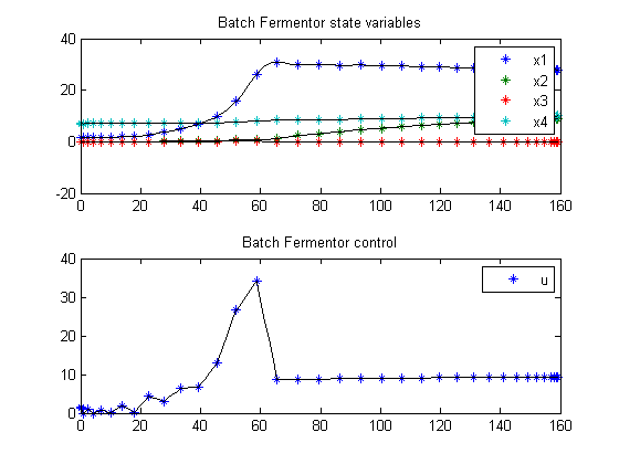
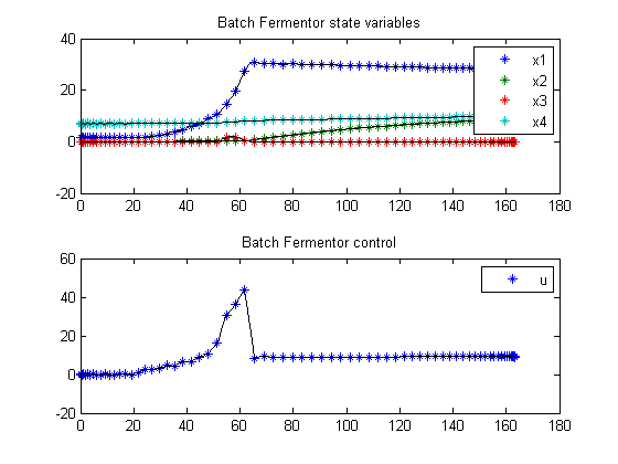
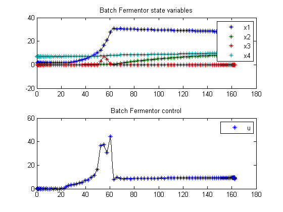
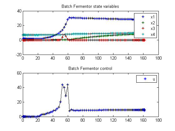
11.3 Plot result
    subplot(2,1,1);
    ezplot([x1; x2; x3; x4]);
    legend('x1','x2','x3','x4');
    title('Batch Fermentor state variables');

    subplot(2,1,2);
    ezplot(u);
    legend('u');
    title('Batch Fermentor control');
    drawnow

    % Copy solution for initializing next round
    x1_init  = subs(x1,solution);
    x2_init  = subs(x2,solution);
    x3_init  = subs(x3,solution);
    x4_init  = subs(x4,solution);
    u_init   = subs(u,solution);
    tf_init  = subs(t_f,solution);

end
« Previous « Start » Next »
