« Previous « Start » Next »
39 Fuller Phenomenon
A Short Introduction to Optimal Control, Ugo Boscain, SISSA, Italy
3.6 Fuller Phenomenon.
39.1 Problem Description
Find u over t in [0; inf ] to minimize:
subject to:
Reference: [7]
39.2 Problem setup
toms t
toms t_f
p = tomPhase('p', t, 0, t_f, 60);
setPhase(p);

tomStates x1 x2
tomControls u

% Initial guess
x0 = {t_f == 10
    icollocate(x1 == 10-10*t/t_f)
    icollocate(x2 == 0)
    collocate(u == -1+2*t/t_f)};

% Box constraints
cbox = {1 <= t_f <= 1e4
    -1 <= collocate(u) <= 1};

% Boundary constraints
cbnd = {initial({x1 == 10; x2 == 0})
    final({x1 == 0; x2 == 0})};

% ODEs and path constraints
ceq = collocate({dot(x1) == x2; dot(x2) == u});

% Objective
objective = integrate(x1.^2);
39.3 Solve the problem
options = struct;
options.name = 'Fuller Phenomenon';
options.solver = 'snopt';
solution = ezsolve(objective, {cbox, cbnd, ceq}, x0, options);
t  = subs(collocate(t),solution);
x1 = subs(collocate(x1),solution);
x2 = subs(collocate(x2),solution);
u  = subs(collocate(u),solution);
Problem type appears to be: con
Starting numeric solver
===== * * * =================================================================== * * *
TOMLAB - Tomlab Optimization Inc. Development license  999001. Valid to 2011-02-05
=====================================================================================
Problem: ---  1: Fuller Phenomenon              f_k     242.423532418144480000
                                       sum(|constr|)      0.000000063718580492
                              f(x_k) + sum(|constr|)    242.423532481863050000
                                              f(x_0)    333.333333333328770000

Solver: snopt.  EXIT=0.  INFORM=1.
SNOPT 7.2-5 NLP code
Optimality conditions satisfied

FuncEv   28 GradEv   26 ConstrEv   27 ConJacEv   26 Iter   14 MinorIter  248
CPU time: 0.218750 sec. Elapsed time: 0.219000 sec.
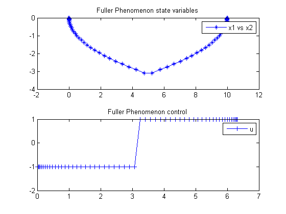
39.4 Plot result
subplot(2,1,1)
plot(x1,x2,'*-');
legend('x1 vs x2');
title('Fuller Phenomenon state variables');

subplot(2,1,2)
plot(t,u,'+-');
legend('u');
title('Fuller Phenomenon control');
« Previous « Start » Next »
