Dynamic optimization of bioprocesses: efficient and robust numerical strategies 2003, Julio R. Banga, Eva Balsa-Cantro, Carmen G. Moles and Antonio A. Alonso
Case Study III: Optimal Drug Scheduling for Cancer Chemotherapy
Many researches have devoted their efforts to determine whether current methods for drugs administration during cancer chemotherapy are optimal, and if alternative regimens should be considered. Martin (1992) considered the interesting problem of determining the optimal cancer drug scheduling to decrease the size of a malignant tumor as measured at some particular time in the future. The drug concentration must be kept below some level throughout the treatment period and the cumulative (toxic) effect of the drug must be kept below the ultimate tolerance level. Bojkov et al. (1993) and Luus et al. (1995) also studied this problem using direct search optimization. More recently, Carrasco and Banga (1997) have applied stochastic techniques to solve this problem, obtaining better results (Carrasco & Banga 1998). The mathematical statement of this dynamic optimization problem is: Find u(t) over t in [t0; t_f ] to maximize:
| J = x1(tf) |
subject to:
| = −k1*x1+k2*(x2−k3)*H(x2−k3) |
| = u−k4*x2 |
| = x2 |
where the tumor mass is given by N = 10^12 * exp (-x1) cells, x2 is the drug concentration in the body in drug units [D] and x3 is the cumulative effect of the drug. The parameters are taken as k1 = 9.9e-4 days, k2 = 8.4e-3 days-1 [De-1], k3 = 10 [De-1], and k4 = 0.27 days-1. The initial state considered is:
| x(t0) = [log(100) 0 0]′ |
where,
H(x2-k3) = 1 if x2 >= k3 or 0 if x2 < k3
and the final time t_f = 84 days. The optimization is subject to the following constraints on the drug delivery (control variable):
| u >= 0 |
There are the following path constraints on the state variables:
| x2(t) <= 50 |
| x3(t) <= 2.1e3 |
Also, there should be at least a 50% reduction in the size of the tumor every three weeks, so that the following point constraints must be considered:
| x1(21) >= log(200) |
| x1(42) >= log(400) |
| x1(63) >= log(800) |
State number 3 is converted to an integral constraints in the formulation.
Reference: [3]
toms t

nn = [20 40 120];

for i = 1:length(nn)
    n = nn(i);
    p = tomPhase('p', t, 0, 84, n);
    setPhase(p);

    tomStates x1 x2
    tomControls u

    % Initial guess
    if i==1
        x0 = {icollocate(x2 == 10)
            collocate(u == 20)};
    else
        x0 = {icollocate({x1 == x1opt; x2 == x2opt})
            collocate(u == uopt)};
    end

    % Box constraints
    cbox = {
        0 <= mcollocate(x1)
        0 <= mcollocate(x2) <= 50
        0 <= collocate(u)   <= 80};

    % Boundary constraints
    cbnd = initial({x1 == log(100); x2 == 0});

    % ODEs and path constraints
    k1 = 9.9e-4; k2 = 8.4e-3;
    k3 = 10;     k4 = 0.27;
    ceq = {collocate({
        dot(x1) == -k1*x1+k2*max(x2-k3,0)
        dot(x2) == u-k4*x2})
        % Point-wise conditions
        atPoints([21;42;63],x1) >= log([200;400;800])
        % Integral constr.
        integrate(x2) == 2.1e3};

    % Objective
    objective = -final(x1);
    options = struct;
    options.name = 'Drug Scheduling';
    options.solver = 'multiMin';
    options.xInit = 130-n;
    solution = ezsolve(objective, {cbox, cbnd, ceq}, x0, options);

    x1opt = subs(x1, solution);
    x2opt = subs(x2, solution);
    uopt  = subs(u, solution);
Problem type appears to be: lpcon
Starting numeric solver
===== * * * =================================================================== * * *
TOMLAB - Tomlab Optimization Inc. Development license  999001. Valid to 2011-02-05
=====================================================================================
Problem: ---  1: Drug Scheduling - Trial 1      f_k     -16.628828853430683000
                                       sum(|constr|)      0.000000000002606145
                              f(x_k) + sum(|constr|)    -16.628828853428075000

Solver: multiMin with local solver snopt.  EXIT=0.  INFORM=0.
Find local optima using multistart local search
Did 1 local tries. Found 1 global, 1 minima. TotFuncEv 1. TotConstrEv 33

FuncEv    1 ConstrEv   33 ConJacEv   32 Iter   15
CPU time: 0.375000 sec. Elapsed time: 0.375000 sec.
Problem type appears to be: lpcon
Starting numeric solver
===== * * * =================================================================== * * *
TOMLAB - Tomlab Optimization Inc. Development license  999001. Valid to 2011-02-05
=====================================================================================
Problem: ---  1: Drug Scheduling - Trial 1      f_k     -16.875588505484753000
                                       sum(|constr|)      0.000000000001656122
                              f(x_k) + sum(|constr|)    -16.875588505483098000

Solver: multiMin with local solver snopt.  EXIT=0.  INFORM=0.
Find local optima using multistart local search
Did 1 local tries. Found 1 global, 1 minima. TotFuncEv 1. TotConstrEv 43

FuncEv    1 ConstrEv   43 ConJacEv   42 Iter   15
CPU time: 0.421875 sec. Elapsed time: 0.422000 sec.
Problem type appears to be: lpcon
Starting numeric solver
===== * * * =================================================================== * * *
TOMLAB - Tomlab Optimization Inc. Development license  999001. Valid to 2011-02-05
=====================================================================================
Problem: ---  1: Drug Scheduling - Trial 1      f_k     -17.395852753239591000
                                       sum(|constr|)      0.000000023567180277
                              f(x_k) + sum(|constr|)    -17.395852729672409000

Solver: multiMin with local solver snopt.  EXIT=0.  INFORM=0.
Find local optima using multistart local search
Did 1 local tries. Found 1 global, 1 minima. TotFuncEv 1. TotConstrEv 53

FuncEv    1 ConstrEv   53 ConJacEv   52 Iter   19
CPU time: 1.875000 sec. Elapsed time: 1.907000 sec.
end
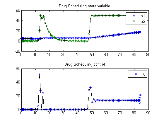
subplot(2,1,1)
ezplot([x1;x2]);
legend('x1','x2');
title('Drug Scheduling state variable');

subplot(2,1,2)
ezplot(u);
legend('u');
title('Drug Scheduling control');