« Previous « Start » Next »
28 Curve Area Maximization
On smooth optimal control determination, Ilya Ioslovich and Per-Olof Gutman, Technion, Israel Institute of Technology.
Example 3: Maximal area under a curve of given length
28.1 Problem Description
Find u over t in [0; 1 ] to minimize:
subject to:
Reference: [18]
28.2 Problem setup
toms t
p = tomPhase('p', t, 0, 1, 20);
setPhase(p);

tomStates x1 x2
tomControls u

x0 = {icollocate({x1 == 0.1, x2 == t*pi/3}), collocate(u==0.5-t)};

% Boundary constraints
cbnd = {initial({x1 == 0; x2 == 0})
    final({x1 == 0; x2 == pi/3})};

% ODEs and path constraints
ceq = collocate({dot(x1) == u
    dot(x2) == sqrt(1+u.^2)});

% Objective
objective = -integrate(x1);
28.3 Solve the problem
options = struct;
options.name = 'Curve Area Maximization';
solution = ezsolve(objective, {cbnd, ceq}, x0, options);
Problem type appears to be: lpcon
Starting numeric solver
===== * * * =================================================================== * * *
TOMLAB - Tomlab Optimization Inc. Development license  999001. Valid to 2011-02-05
=====================================================================================
Problem: ---  1: Curve Area Maximization        f_k      -0.090586073472539108
                                       sum(|constr|)      0.000000003581094695
                              f(x_k) + sum(|constr|)     -0.090586069891444410
                                              f(x_0)     -0.099999999999999756

Solver: snopt.  EXIT=0.  INFORM=1.
SNOPT 7.2-5 NLP code
Optimality conditions satisfied

FuncEv    1 ConstrEv  120 ConJacEv  120 Iter   99 MinorIter  137
CPU time: 0.171875 sec. Elapsed time: 0.188000 sec.
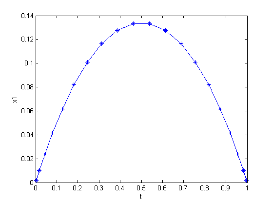
28.4 Plot result
t = subs(collocate(t),solution);
x1 = subs(collocate(x1),solution);
figure(1);
plot(t,x1,'*-');
xlabel('t')
ylabel('x1')
« Previous « Start » Next »
