« Previous « Start » Next »
2 Overall Design
The scope of TOMLAB is large and broad, and therefore there is a
need of a well-designed system. It is also natural to use the
power of the Matlab language, to make the system flexible and
easy to use and maintain. The concept of structure arrays is used
and the ability in Matlab to execute Matlab code defined as
string expressions and to execute functions specified by a string.
2.1 Structure Input and Output
Normally, when solving an optimization problem, a direct call to a
solver is made with a long list of parameters in the call. The
parameter list is solver-dependent and makes it difficult to make
additions and changes to the system.
TOMLAB solves the problem in two steps. First the problem is defined
and stored in a Matlab structure. Then the solver is called with a
single argument, the problem structure. Solvers that were not
originally developed for the TOMLAB environment needs the usual long
list of parameters. This is handled by the driver routine
tomRun.m which can call any available solver, hiding the
details of the call from the user. The solver output is collected in
a standardized result structure and returned to the user.
2.2 Introduction to Solver and Problem Types
TOMLAB solves a number of different types of optimization problems.
The currently defined types are listed in Table
2.2.
The global variable
probType contains the current type of
optimization problem to be solved.
An optimization solver is defined
to be of type
solvType , where
solvType is any of the
probType entries in Table
2.2.
It is clear that a
solver of a certain
solvType is able to solve a problem defined
to be of another type.
For example, a constrained nonlinear
programming solver should be able to solve unconstrained problems,
linear and quadratic programs and constrained nonlinear least squares
problems.
In the graphical user interface and menu system an
additional variable
optType is defined to keep track of what
type of problem is defined as the main subject. As an example, the
user may select the type of optimization to be quadratic programming
(
optType == 2), then select a particular problem that is a
linear programming problem (
probType == 8) and then as the
solver choose a constrained NLP solver like MINOS (
solvType ==
3).
| The different types of optimization problems defined in TOMLAB . |
|
| probType |
|
Type of optimization problem |
|
| uc |
1 |
Unconstrained optimization (incl. bound constraints). |
| qp |
2 |
Quadratic programming. |
| con |
3 |
Constrained nonlinear optimization. |
| ls |
4 |
Nonlinear least squares problems (incl. bound constraints). |
| lls |
5 |
Linear least squares problems. |
| cls |
6 |
Constrained nonlinear least squares problems. |
| mip |
7 |
Mixed-Integer programming. |
| lp |
8 |
Linear programming. |
| glb |
9 |
Box-bounded global optimization. |
| glc |
10 |
Global mixed-integer nonlinear programming. |
| miqp |
11 |
Constrained mixed-integer quadratic programming. |
| minlp |
12 |
Constrained mixed-integer nonlinear optimization. |
| lmi |
13 |
Semi-definite programming with Linear Matrix Inequalities. |
| bmi |
14 |
Semi-definite programming with Bilinear Matrix Inequalities. |
| exp |
15 |
Exponential fitting problems. |
| nts |
16 |
Nonlinear Time Series. |
| lcp |
22 |
Linear Mixed-Complimentary Problems. |
| mcp |
23 |
Nonlinear Mixed-Complimentary Problems. |
|
Please note that since the actual numbers used for
probType may
change in future releases, it is recommended to use the text
abbreviations. See help for
checkType for further information.
Define
probSet to be a set of defined optimization problems
belonging to a certain class of problems of type
probType .
Each
probSet is physically stored in one file, an
Init File. In
Table
2.2 the currently defined problem sets are listed, and
new
probSet sets are easily added.
| Defined test problem sets in TOMLAB . probSets marked with * are not part of the standard distribution |
|
| probSet |
probType |
Description of test problem set |
|
| uc |
1 |
Unconstrained test problems. |
| qp |
2 |
Quadratic programming test problems. |
| con |
3 |
Constrained test problems. |
| ls |
4 |
Nonlinear least squares test problems. |
| lls |
5 |
Linear least squares problems. |
| cls |
6 |
Linear constrained nonlinear least squares problems. |
| mip |
7 |
Mixed-integer programming problems. |
| lp |
8 |
Linear programming problems. |
| glb |
9 |
Box-bounded global optimization test problems. |
| glc |
10 |
Global MINLP test problems. |
| miqp |
11 |
Constrained mixed-integer quadratic problems. |
| minlp |
12 |
Constrained mixed-integer nonlinear problems. |
| lmi |
13 |
Semi-definite programming with Linear Matrix Inequalities. |
| bmi |
14 |
Semi-definite programming with Bilinear Matrix Inequalities. |
| exp |
15 |
Exponential fitting problems. |
| nts |
16 |
Nonlinear time series problems. |
| lcp |
22 |
Linear mixed-complimentary problems. |
| mcp |
23 |
Nonlinear mixed-complimentary problems. |
| |
| mgh |
4 |
More, Garbow, Hillstrom nonlinear least squares problems. |
| chs* |
3 |
Hock-Schittkowski constrained test problems. |
| uhs* |
1 |
Hock-Schittkowski unconstrained test problems. |
| cto* |
3 |
CUTE constrained test problems as dll-files. |
| ctl* |
3 |
CUTE large constrained test problems as dll-files. |
| uto* |
1 |
CUTE unconstrained test problems as dll-files. |
| utl* |
1 |
CUTE large unconstrained test problems as dll-files. |
|
The names of the predefined Init Files that do the problem setup,
and the corresponding low level routines are constructed as two
parts. The first part being the abbreviation of the relevant
probSet , see Table
2.2, and the second part denotes
the computed task, shown in Table
2.2. The user normally
does not have to define the more complicated functions
◇_d2c and
◇_d2r. It is recommended to
supply this information when using solver which require second order
information, such as TOMLAB /KNITRO and TOMLAB /CONOPT.
Names for predefined Init Files and low level m-files in TOMLAB . |
|
| Generic name |
Purpose ( ◇ is any probSet,
e.g. ◇=con) |
|
◇_prob |
Init File that either defines a
string matrix with problem names or
a structure prob for the selected problem. |
| ◇_f |
Compute objective function f(x). |
| ◇_g |
Compute the gradient vector g(x). |
| ◇_H |
Compute the Hessian matrix H(x). |
| ◇_c |
Compute the vector of constraint functions c(x). |
| ◇_dc |
Compute the matrix of constraint normals, ∂ c(x) /dx. |
| ◇_d2c |
Compute the 2nd part of
2nd derivative matrix of the Lagrangian function,
Σi λi ∂2 ci(x) / dx2. |
| ◇_r |
Compute the residual vector r(x). |
| ◇_J |
Compute the Jacobian matrix J(x). |
| ◇_d2r |
Compute the 2nd part of the Hessian matrix, Σi ri(x) ∂2 ri(x) / dx2 |
|
The Init File has two modes of operation; either return a string
matrix with the names of the problems in the
probSet or a
structure with all information about the selected problem. All
fields in the structure, named
Prob , are presented in tables
in Section
A. Using a structure makes it easy to add
new items without too many changes in the rest of the system. The
menu systems and the GUI are using the string matrix returned from
the Init File for user selection of which problem to be solved.
For further discussion about the definition of optimization
problems in TOMLAB , see Section
4.
There are default values for everything that is possible to set defaults for,
and all routines are written in a way that makes it possible for the user to
just set an input argument empty and get the default.
2.3 The Process of Solving Optimization Problems
A flow-chart of the process of optimization in TOMLAB is shown in
Figure
1. It is inefficient to use an interactive
system. This is symbolized with the
Standard User box in the
figure, which directly runs the
Optimization Driver,
tomRun . If a problem is specified in the TOMLAB format and not
converted to the TOMLAB Init File, then the GUI and menu systems are not
available and the user must either call the driver routine or call
the solver directly. The direct solver call is possible for all
TOMLAB solvers, if the user has executed
ProbCheck prior to
the call. See Section
3 for a list of the TOMLAB
solvers.
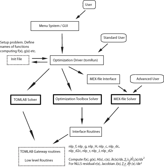
Figure 1: The process of optimization in TOMLAB .
Depending on the type of problem, the user needs to supply the
low-level routines that calculate the objective function,
constraint functions for constrained problems, and also if
possible, derivatives. To simplify this coding process so that the
work has to be performed only once, TOMLAB provides
gateway
routines that ensure that any solver can obtain the values in the
correct format.
For example, when working with a least squares problem, it is natural
to code the function that computes the vector of residual functions
ri(
x1,
x2,…), since a dedicated least squares solver probably
operates on the residual while a general nonlinear solver needs a
scalar function, in this case
f(
x) = 1/2
rT(
x)
r(
x). Such
issues are automatically handled by the gateway functions.
2.4 Low Level Routines and Gateway Routines
Low level routines are the routines that compute:
-
The objective function value
- The gradient vector
- The Hessian matrix (second derivative matrix)
- The residual vector (for nonlinear least squares problems)
- The Jacobian matrix (for nonlinear least squares problems)
- The vector of constraint functions
- The matrix of constraint normals (the constraint Jacobian)
- The second part of the second derivative of the Lagrangian function.
The last three routines are only needed for constrained
problems.
The names of these routines are defined in the structure fields
Prob.FUNCS.f ,
Prob.FUNCS.g ,
Prob.FUNCS.H etc. It
is the task for the
Assign routine to set the names of the
low level m-files. This is done by a call to the routine
conAssign with the names as arguments for example. There are
Assign routines for all problem types handled by TOMLAB . As an
example, see 'help conAssign' in MATLAB.
 Prob = conAssign('f', 'g', 'H', HessPattern, x_L, x_U, Name,x_0,...
        pSepFunc, fLowBnd, A, b_L, b_U, 'c', 'dc', 'd2c', ConsPattern,...
        c_L, c_U, x_min, x_max, f_opt, x_opt);
Only the low level routines relevant for a certain type of
optimization problem need to be coded. There are dummy routines
for the others. Numerical differentiation is automatically used
for gradient, Jacobian and constraint gradient if the
corresponding user routine is non present or left out when calling
conAssign . However, the solver always needs more time to
estimate the derivatives compared to if the user supplies a code
for them. Also the numerical accuracy is lower for estimated
derivatives, so it is recommended that the user always tries to
code the derivatives, if it is possible. Another option is
automatic differentiation with TOMLAB /MAD.
TOMLAB uses gateway routines (
nlp_f ,
nlp_g ,
nlp_H ,
nlp_c ,
nlp_dc ,
nlp_d2c ,
nlp_r ,
nlp_J ,
nlp_d2r ). These routines
extract the search directions and line search steps, count
iterations, handle separable functions, keep track of the kind of
differentiation wanted etc. They also handle the separable NLLS
case and NLLS weighting. By the use of global variables,
unnecessary evaluations of the user supplied routines are avoided.
To get a picture of how the low-level routines are used in the system,
consider Figure
2 and
3.
Figure
2 illustrates the chain of calls when
computing the objective function value in
ucSolve for a nonlinear
least squares problem defined in
mgh_prob ,
mgh_r and
mgh_J .
Figure
3 illustrates the chain of calls when
computing the numerical approximation of the gradient (by use of the
routine
fdng ) in
ucSolve
for an unconstrained problem defined in
uc_prob and
uc_f .
ucSolve <==> nlp_f <==> ls_f <==> nlp_r <==> mgh_r
Figure 2: The chain of calls when computing the objective function value in
ucSolve for a nonlinear least squares problem defined in mgh_prob ,
mgh_r and mgh_J .
ucSolve <==> nlp_g <==> fdng <==> nlp_r <==> uc_f
Figure 3: The chain of calls when
computing the numerical approximation of the gradient in ucSolve
for an unconstrained problem defined in uc_prob and uc_f .
Information about a problem is stored in the structure variable
Prob , described in detail in the tables in Appendix
A. This variable is an argument to all low level
routines. In the field element
Prob.user , problem specific
information needed to evaluate the low level routines are stored.
This field is most often used if problem related questions are asked
when generating the problem. It is often the case that the user
wants to supply the low-level routines with additional information
besides the variables
x that are optimized. Any unused fields
could be defined in the structure
Prob for that purpose. To
avoid potential conflicts with future TOMLAB releases, it is
recommended to use subfields of
Prob.user . It the user wants
to send some variables a, B and C, then, after creating the
Prob structure, these extra variables are added to the
structure:
Prob.user.a=a;
Prob.user.B=B;
Prob.user.C=C;
Then, because the
Prob structure is sent to all low-level
routines, in any of these routines the variables are picked out from
the structure:
a = Prob.user.a;
B = Prob.user.B;
C = Prob.user.C;
A more detailed description of how to define new problems is given
in sections
5,
6 and
8.
The usage of
Prob.user is described in Section
14.2.
Different solvers all have different demand on how
information should be supplied, i.e. the function to optimize, the gradient
vector, the Hessian matrix etc. To be able to code the problem only once, and
then use this formulation to run all types of solvers,
interface routines that returns information in the format needed
for the relevant solver were developed.
Table
1 describes the low level test functions and the
corresponding Init File routine needed for the predefined constrained
optimization (
con) problems. For the predefined unconstrained
optimization (
uc) problems, the global optimization (
glb, glc)
problems and the quadratic programming problems (
qp) similar
routines have been defined.
Table 1: Generally constrained nonlinear (con) test problems.
|
| Function |
Description |
|
| con_prob |
Init File. Does the
initialization of the con test problems. |
| con_f |
Compute the objective function f(x) for con test problems. |
| con_g |
Compute the gradient g(x) for con test problems.
x |
| con_H |
Compute the Hessian matrix H(x) of f(x) for con test problems. |
| con_c |
Compute the constraint residuals c(x) for con test problems. |
| con_dc |
Compute the derivative of the constraint residuals for con test problems. |
| con_d2c |
Compute the 2nd part of
2nd derivative matrix of the Lagrangian function,
Σi λi ∂2 ci(x) / dx2
for con test problems. |
| con_fm |
Compute merit function θ(xk). |
| con_gm |
Compute gradient of merit function θ(xk). |
|
To conclude, the system design is flexible and easy to expand
in many different ways.
« Previous « Start » Next »
