« Previous « Start » Next »
10 tomGUI - The Graphical User Interface
The Graphical User Interface is started by calling the Matlab
m-file
tomlabGUI.m , i.e. by entering the command
tomlabGUI at the Matlab prompt. There is a short command
tomGUI.m . The GUI has five modes; Normal (Result mode),
Figure, General parameter mode, Solver parameter mode and Plot
parameter mode. At start the GUI is in Normal mode, shown in Figure
5.
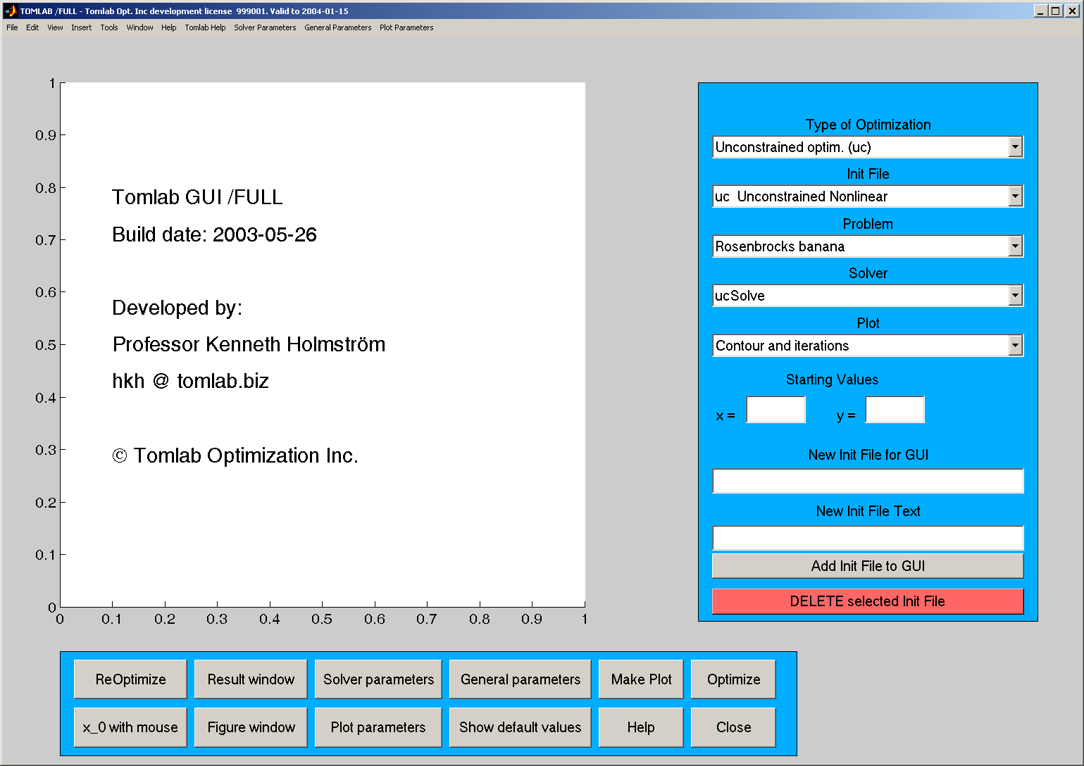
Figure 5: The GUI after startup.
There are one axes area,
five menus;
Type of Optimization,
Init File,
Problem,
Solver and
Plot, and
twelve push buttons;
ReOptimize, x0 with Mouse, Result window, Figure window,
Solver parameters, Plot parameters, General parameters, Show default
values, Make Plot, Help, Optimize and
Close.
There are two edit controls where it is possible to enter the first
two initial values (Starting Values) of the unknown parameters
vector. If the problem has more then two dimensions, the rest of the
initial values are given in the
General Parameter mode.
In the axes area plots and information given as text are displayed.
The
Type of Optimization menu is used to select subject, i.e.
which type of problem to be solved. There are currently ten main
problem types; unconstrained optimization, quadratic programming,
constrained optimization, nonlinear least squares, exponential sum
fitting, constrained nonlinear least squares, mixed-integer linear
programming, linear programming, global unconstrained optimization
and global constrained optimization.
With the selection in the
Init File, the user makes the choice
of which file to get the problem to solve from. In the
Problem
menu, the user selects the actual problem to be solved, among the
ones present in the current selected Init File. Presently, there are
about 15 to 50 predefined test problems for each problem type.
The user can easily define his own problems and try to solve them
using any solver, see sections
5,
6 and
8.
The
Solver menu is used to select solver. It can either be a
TOMLAB internal solver, a solver in the Matlab Optimization
Toolbox or a general-purpose solver implemented in Fortran or C and
ran using a MEX-file interface.
Changing
Type of Optimization will automatically change the
menu entries in the
Init File menu, the
Problem menu,
and the
Solver menu.
From the
Plot menu, the type of plot to be drawn is selected.
The different types are contour plot, mesh plot, plot of function
values and plot of convergence rate. The contour plot and the mesh
plot can be displayed either in the axes area or in a new figure.
The plot of function values and convergence rate are always
displayed in a new figure. For least squares problems and
exponential fitting problems it is possible to plot the residuals,
the starting model and the obtained model.
When clicking the
Show default values button, the default
values for every parameter are displayed in the edit controls. The
button then shows the text
Hide default values. If pushing the
button again, the parameters will disappear. Before solving a
problem, the user can change any of the values. If leaving an edit
control empty, the default values are used. If giving a value less
than -1, it will normally not be used at all. The default values are
used instead. The value −999 indicates missing value, and the
default value is always used by the solver. The value −900
indicates both a missing value, and that this quantity is never used
by the currently defined solver. Thus it is pointless to set a value
for this quantity.
The buttons
General Parameters,
Solver Parameters
and
Plot Parameters
are described in Section
10.1.
Pushing the
Make Plot
button gives a plot of the current problem.
Pushing the
Figure window
button switches back to the last plot made.
In the contour
plot, known local minima, known local maxima and known saddle points are
shown. It is possible to make a contour plot and a mesh plot without first
solving the problem. After the problem is solved, a contour plot shows the
search direction and trial step lengths for each iteration. A contour plot
of the classical Rosenbrock banana function, together with the iteration
search steps and with marks for the line search trials displayed, is shown
in Figure
6.
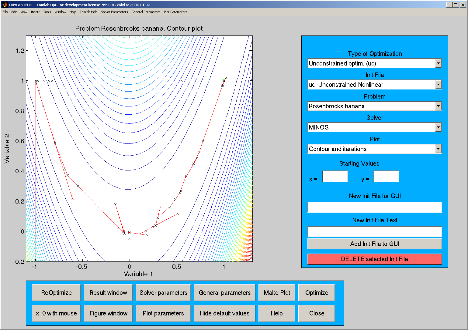
Figure 6: A contour plot with the search directions and marks for
the line search trials for each iteration when solving an
unconstrained optimization problem.
A contour plot for a constrained problem and a plot of the data
is given in
Figure
7.
In the contour plot, (inequality) constraints are depicted as dots.
Starting from the infeasible point (
x1,
x2)=(−5.0,2.5), the solution
algorithm first finds a point inside the feasible region. The algorithm then
iteratively finds new points. For several of the search directions, the full
step is too long and violates one of the constraints. Marks show the line
search trials. Finally, the algorithm converges to the optimal solution (
x1*,
x2*)=(−9.5474,1.0474).
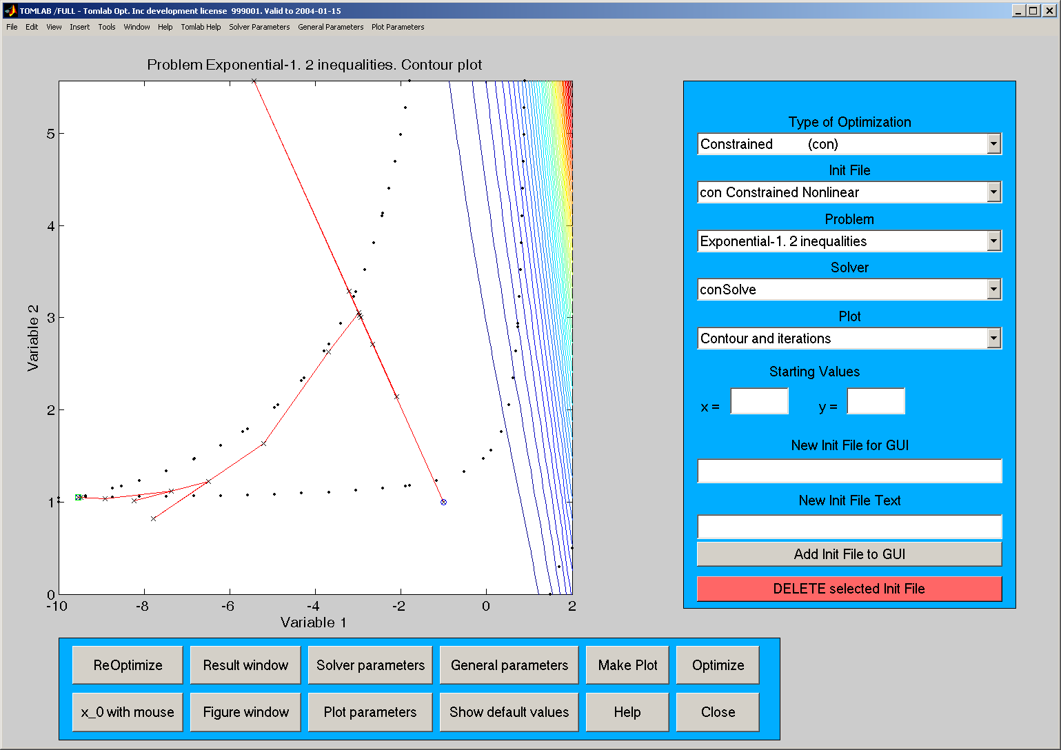
Figure 7: A contour plot for a constrained problem
In Figure
8
is shown
a plot of the data and the
obtained model for a nonlinear least squares problem,
in this case an exponential fitting problem.
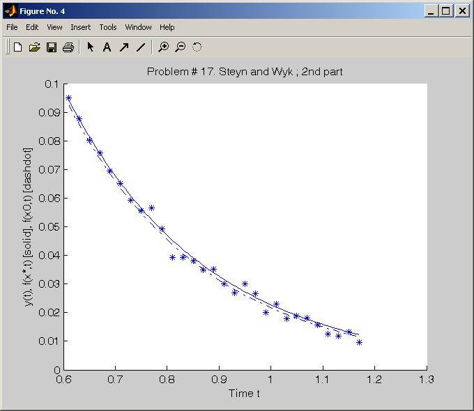
Figure 8: A plot of the data and the model for a exponential sum fitting
problem. The figure shows the second part of the data series and the
estimated optimal model
For global optimization one option is
a contour plot together with the sampled points. This plot is
illustrative for how the search procedure is sampling.
The points samples cluster around the different local minima.
One example is shown in
Figure
9, where the blue dots are the sampled points.
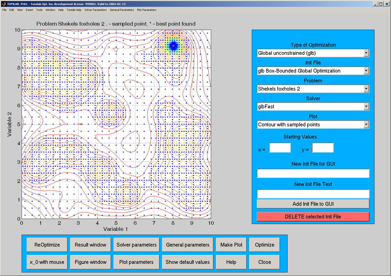
Figure 9: Contour plot with sampled points for the two-dimensional
Shekels foxhole problem.
The problem has several local optima and is best solved
by global optimization
methods.
The
Help
button gives some information about the current problem, e.g. the
number of variables.
Note that there are four drag menus on top
TOMLAB Help,
Solver Parameters,
General Parameters,
and
Plot Parameters.
Selecting any items in these menus displays a help text in plot window.
When the user has chosen a solver and a problem, he then pushes the
Optimize
button to solve it. When the algorithm has converged, information about the
solution procedure are displayed. This information will include the solution
found, the function value at the solution, the number of iterations used,
the number of function evaluations, the number of gradient evaluations, the
number of floating point operations used and the computation time. If no
algorithm is selected as in Figure
5, the Run button has the same
function as the Plot button.
If a contour plot is
displayed in the axes area and the user pushes the button named
x_0 with mouse, it is
possible to select starting point for the current algorithm using the mouse.
Pushing the
ReOptimize
button, the current problem is re-optimized with the
starting point defined as the solution found in the previous solution attempt.
To close the GUI, push the Close button.
10.1 The Input Modes
This section describes the three input modes
General
Parameter mode,
Solver Parameter mode and
Plot
Parameter mode. When pushing one of these buttons, the GUI will
change to the corresponding mode. The axes area is replaced by
more edit controls and menus.
10.2 General Parameter Mode
The General Parameter Mode makes it possible to
set parameters common for the current
Type of Optimization given,
See Figure
10.
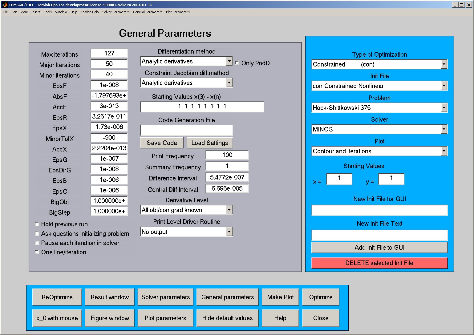
Figure 10: The GUI in General Parameter Mode.
To the left is the maximum number of iterations
(
Max iterations), and limits on major and minor iterations.
The last two are used for some solvers.
Above each other is the tolerances, e.g. the
termination tolerance on the function
value (EpsF),
the rank test tolerance
(EpsR),
the termination tolerance on the change
in the decision variables (EpsX),
and the termination tolerance on the gradient (EpsG).
If a solver for constrained optimization handling linear constraints
is selected, an edit control
for the allowed tolerance on constraint violation (EpsB) is shown.
Another similar edit control (EpsC) is shown for solvers handling
nonlinear constraints.
This edit control sets
the allowed termination tolerance on the
nonlinear constraint violation.
For problems with more than two decision variables, starting
values for decision variable
x3 to
xn are given in the
edit control named 'Starting Values x3 - xn'. Starting values for
x1 and
x2 are given in the edit controls named
'Starting Values'.
The first menu selects method to compute first and second
derivatives. Except for using an analytical expression, these can be
computed either by automatic differentiation using the MAD toolbox,
or by five different approaches for numerical differentiation. Three
of them requires the Spline Toolbox to be installed.
The
Print Level Driver Routine menu selects the level of
output from the optimization driver after the solver has been
called. All this output is printed in the Matlab Command Window.
Normally it is enough with the default information given in the
GUI result window.
If the
Pause Each Iteration check box is selected, the TOMLAB
internal solvers are using the pause statement to halt after each
iteration.
If the check box
Hold Previous Run is selected, all information about the
runs are stored. Making a contour plot, the step and trial step lengths for all
solution attempts are drawn. This option is useful, e.g. when comparing the
performance of different algorithms or checking how the choice of starting
point affects the solution procedure.
For some predefined test problems, it is possible to set parameter
values when initializing the problem. These parameters can for
example be the size of the problem, the number of residuals or the
number of constraints. Questions asking for input of the
parameters will appear when selecting the check box named
Ask
Questions when defining problem, otherwise, if the check box is
not selected, default values will be used.
When selecting exponential fitting problems, two new menus and a
new edit control will appear. The number of exponential terms
(
Terms) in the approximating model is selected, default two.
There is a choice whether to solve the weighted least squares
fitting problem using an ordinary or separable nonlinear least
squares algorithm (
Least Squares Method). There are four
types of residual weighting selectable (
Residual Weights).
The option
y-weighting, i.e. weighting with the measured
data, is often proposed, but default is
No weighting.
Code Generation
Entering a name in the edit control
Code Generation File and
clicking the
Save Code button, two files will be generated;
one Matlab mat-file and one Matlab m-file. The file name given
should not include any extension. For example, entering the name
test in the edit control, the files
test.mat and
test.m will be generated. The files are saved in the
current directory. In the mat-file parameters are stored in the
Prob structure format, but the name of the structure is
Problem . In the m-file all commands needed to make a
stand-alone run without using the GUI are defined. The parameter
values are those currently used by the GUI. To run the problem, just
issue
test in the command window. Note that the print level is
set very low by default, and often nothing is displayed. It is easy
to edit the m-file for different needs.
If entering a name in the
Code Generation File edit control
and clicking the
Load Settings button, the GUI will read the
corresponding mat-file. The mat-file should contain a TOMLAB
Prob structure with the name
Problem . This is the
type of mat-file generated by the
Save Code button. The GUI
will switch to the
Type of Optimization,
Init File,
Problem File and
Solver defined in the mat-file. The
default values for all parameters will be loaded from the
mat-file. This option is useful for retrieving complicated
settings for a particular problem and solver.
10.3 Solver Parameter Mode
For the Solver Parameter Mode the parameters areas shown, and
possible to set, are dependent on the particular solver selected
in the
Solver menu. Some parameters are common for many of
the internal TOMLAB solvers FLow, the best guess on a lower bound
for the optimal function value, is used by TOMLAB solver algorithms
using the Fletcher line search algorithm [
23]. In Figure
11 the Solver Parameter Mode for the MINOS solver is
shown. MINOS and SNOPT are the solvers with most parameters to be
set. Default values are always defined, and in the picture is
shown the default values for MINOS.
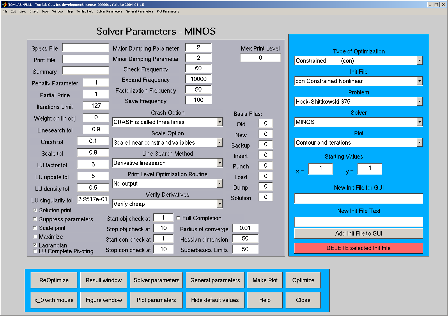
Figure 11: The Solver Parameters for the MINOS solver.
Algorithms using a line search approach needs the line search
accuracy σ (Sigma) between zero and one. Values close to
one (0.9) gives an inaccurate line search, often recommended.
Values close to zero (0.1) gives a more accurate line search,
recommended for conjugate gradient methods and sometimes for
quasi-Newton methods. Another menu determines if a quadratic or a
cubic interpolation shall be used in the line search algorithm.
The
Print Level Optimization Routine menu is used to select
the level of output from the optimization solver. All output
printed during the optimization are displayed in the Matlab
Command Window.
The menu named
Algorithm differs between different solvers.
Some solvers have only one algorithm alternative, others have several.
The menu named
Method also differs between different solvers,
and is sometimes hidden.
Using an unconstrained solver, a least squares solver or an exponential fitting
solver, the menu selects method to compute the search direction. In the
constrained case, the Method menu gives the quadratic programming solver to be
used in SQP algorithms.
10.4 Plot Parameter Mode
The Plot Parameter Mode makes it possible to
set parameters common for plotting,
see Figure
12.
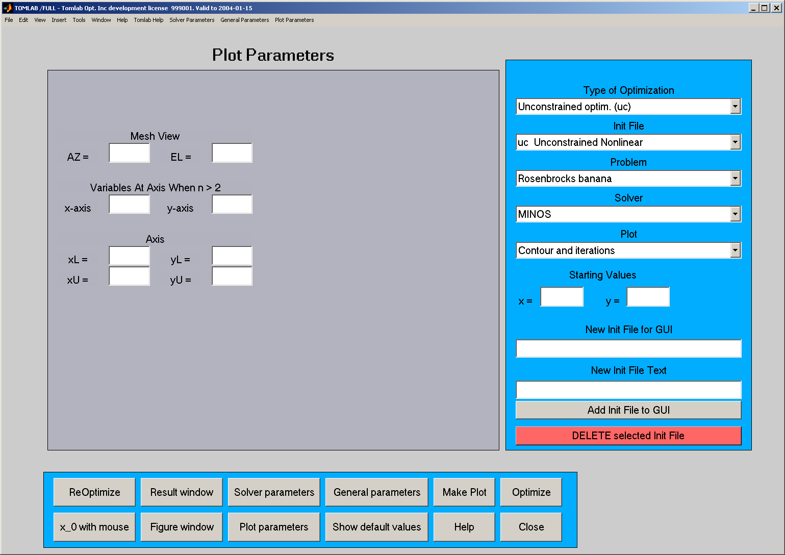
Figure 12: The plot parameters in the Plot Parameter Mode.
The edit controls named 'Axes' set
the axes in the contour plot and the mesh plot.
To make a contour plot or a mesh
plot for problems with more than two decision variables, the user selects the
two-dimensional subspace to plot. The indices of the decision variables
defining the subspace are given in the edit controls called 'Variables At Axis
When
n>2'. The view for a mesh plot is changed using the edit controls 'Mesh
View'.
10.5 tomRemote and tomMenu - The Menu Programs
The general menu program
tomMenu has much of the
functionality of the GUI (Section
10), and is sometimes
faster to use.
tomRemote is possible to run when not running a window
system, e.g. when using telnet to a machine, in which case the GUI
or
tomMenu are not possible to use. Some specific solver
parameter settings are not available in
tomMenu and
tomRemote , as well as the code generation possibility.
tomMenu is described briefly in Section
5.1.4.
Starting the remote menu system, the first menu, seen in Figure
13, is the selection of the type of optimization
problem (
probType).
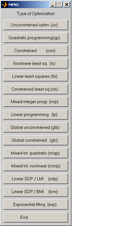
Figure 13: The choice of the Type of Optimization in
tomRemote .
The
tomRemote sub-menu for unconstrained optimization is
shown in Figure
14. The other sub-menus look
similar, with additional items corresponding to options needed for
the relevant problem and solver type. In the following of this
section, the most important standard menu choices are commented.
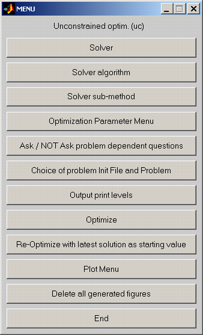
Figure 14: The main menu for unconstrained optimization in
tomRemote .
The
Choice of Problem Init File and Problem button selects the problem
Init File and the problem to be solved. Correspondingly, the
Solver,
Solver algorithm and
Solver sub-method
buttons selects the solver, particular solver algorithm, and other
method choice to be used.
From the
Optimization Parameter Menu, parameters needed for
the solution can be changed. The user selects new values or simply
uses the default values. The parameters are those stored in the
optParam structure, see Table
A. The
Output print levels button selects the level of output to
be displayed in the Matlab Command Window during the solution
procedure. The
Optimization Parameter Menu also allows the
user to choose the differentiation strategy he wants to use.
The
Optimization Parameter Menu is dependent on the type
of optimization problem. A short parameter menu for quadratic
programming is shown in Figure
15.
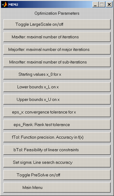
Figure 15: Setting optimization parameters for quadratic
programming.
Pushing the
Optimize button, the relevant routines are called
to solve the problem.
When the problem is solved, it is possible to make different types of plots to
illustrate the solution procedure. Pushing the
Plot Menu button, a
menu choosing type of plot will appear. A overview of the available plotting
options are given in connection with the Graphical User Interface described in
Section
10.
The menu routine is started by just typing
tomMenu at the
Matlab prompt. In Section
5.1 we illustrate how to use the
menu system for linear programming problems (
lpMenu ). The
menus for nonlinear problems work in a similar way.
Calling
tomRemote ) by typing
Result = tomRemote will
return a structure array containing the
Result structures of
all the runs made. As an example, to display the results from the
third run, enter the command
Result(3) . To display the
solution found in the third run, enter the command
Result(3).x_k . The information stored in the structure are
given in Table
B.
The menu program calls the driver routine
tomRun .
There are some options in the menu programs to display graphical
information for the selected problem. For two-dimensional
nonlinear unconstrained problems, the menu programs support
graphical display of the relevant optimization problem as mesh or
contour plots. In the contour plot, the iteration steps are
displayed. For higher-dimensional problems, iterations steps are
displayed in two-dimensional subspaces. Special plots for
nonlinear least squares problems, such as plotting model against
data, are available. The plotting utility also includes plot of
convergence rate, plot of circles approximating points in the
plane for the Circle Fitting Problem etc. The plot facilities are
exactly the same as for the GUI. See Section
10 for
figures similar to the ones produced running the menu system.
10.6 tomHelp - The Help Program
tomHelp is a graphical interface for quick help on all
problem types defined in TOMLAB The interface is started by
entering
tomHelp in the MATLAB command prompt. The menu
system will be displayed as in Figure
16.
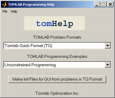
Figure 16: tomHelp start menu.
If a specific problem category is selected then a new menu is
displayed. Text help in the MATLAB command window is displayed by
choosing help from the interface. It is recommended that the
individual demo files are viewed to get an understanding about the
specific problem. The files can be used as a starting point for
defining problem in the TOMLAB format.
The llsDemo menu is illustrated below in Figure
17
Figure 17: llsDemo menu.
« Previous « Start » Next »
