« Previous « Start » Next »
11 TOMLAB Solver Reference
Detailed descriptions of the TOMLAB solvers, driver routines and
some utilities are given in the following sections. Also see the
M-file help for each solver. All solvers except for the TOMLAB Base
Module are described in separate manuals.
11.1 TOMLAB Base Module
For a description of solvers called using the MEX-file interface,
see the M-file help, e.g. for the MINOS solver
minosTL.m . For
more details, see the User's Guide for the particular solver.
Purpose
Solves dense and sparse nonlinear least squares optimization
problems with linear inequality and equality constraints and simple
bounds on the variables.
clsSolve solves problems of the form
|
|
|
f(x) |
= |
|
|
|
| s/t |
xL |
≤ |
x |
≤ |
xU |
| |
bL |
≤ |
Ax |
≤ |
bU |
|
where
x,
xL,
xU R n
R n,
r(
x)
R N,
A Rm1× n and
bL,
bU R
m1.
Calling Syntax
Result = clsSolve(Prob, varargin)
Result = tomRun('clsSolve', Prob);
Description of Inputs
| Prob |
Problem description structure. The following fields are used: |
| |
| Prob |
Problem description structure. The following fields are used:, continued |
| |
| |
Solver.Alg |
Solver algorithm to be run: |
| |
|
0: Gives default, the Fletcher - Xu hybrid method; |
| |
|
1: Fletcher - Xu hybrid method; Gauss-Newton/BFGS. |
| |
|
2: Al-Baali - Fletcher hybrid method; Gauss-Newton/BFGS. |
| |
|
3: Huschens method. SIAM J. Optimization. Vol 4, No 1, pp 108-129 jan 1994. |
| |
|
4: The Gauss-Newton method. |
| |
|
5: Wang, Li, Qi Structured MBFGS method. |
| |
|
6: Li-Fukushima MBFGS method. |
| |
|
7: Broydens method. |
| |
| |
|
Recommendations: Alg=5 is theoretically best, and seems best in practice as
well. Alg=1 and Alg=2 behave very similar, and are robust methods.
Alg=4 may be good for ill-conditioned problems.
Alg=3 and Alg=6 may sometimes fail.
Alg=7 tries to minimize Jacobian evaluations, but might need more
residual evaluations. Also fails more often that other algorithms.
Suitable when analytic Jacobian is missing and evaluations of the Jacobian
is costly. The problem should not be too ill-conditioned. |
| |
| |
Solver.Method |
Method to solve linear system: |
| |
|
0: QR with pivoting (both sparse and dense). |
| |
|
1: SVD (dense). |
| |
|
2: The inversion routine (inv) in Matlab (Uses QR). |
| |
|
3: Explicit computation of pseudoinverse, using pinv(Jk). |
| |
| |
|
Search method technique (if Prob.LargeScale = 1, then Method = 0 always):
Prob.Solver.Method = 0 Sparse iterative QR using Tlsqr. |
| |
| |
LargeScale |
If = 1, then sparse iterative QR using Tlsqr is
used to find search directions |
| |
| |
x_0 |
Starting point. |
| |
x_L |
Lower bounds on the variables. |
| |
x_U |
Upper bounds on the variables. |
| |
| |
b_L |
Lower bounds on the linear constraints. |
| |
b_U |
Upper bounds on the linear constraints. |
| |
A |
Constraint matrix for linear constraints. |
| |
| |
c_L |
Lower bounds on the nonlinear constraints. |
| |
c_U |
Upper bounds on the nonlinear constraints. |
| |
| |
f_Low |
A lower bound on the optimal function value, see LineParam.fLowBnd below. |
| |
| |
SolverQP |
Name of the solver used for QP subproblems. If empty,
the default solver is used. See GetSolver.m and tomSolve.m. |
| |
| |
PriLevOpt |
Print Level. |
| |
optParam |
Structure with special fields for optimization parameters, see Table A. Fields used are:
bTol , eps_absf , eps_g , eps_Rank , eps_x ,
IterPrint , MaxIter , PreSolve , size_f , size_x ,
xTol , wait ,
and
QN_InitMatrix (Initial Quasi-Newton matrix, if not empty, otherwise use identity matrix). |
| |
LineParam |
Structure with line search parameters. Special fields used: |
| |
LineAlg |
If Alg=7 |
| |
|
0 = Fletcher quadratic interpolation line search |
| |
|
3 = Fletcher cubic interpolation line search |
| |
|
otherwise Armijo-Goldstein line search (LineAlg == 2) |
| |
| |
|
If Alg!=7 |
| |
|
0 = Fletcher quadratic interpolation line search |
| |
|
1 = Fletcher cubic interpolation line search |
| |
|
2 = Armijo-Goldstein line search |
| |
|
otherwise Fletcher quadratic interpolation line search (LineAlg == 0) |
| |
| |
|
If Fletcher, see help LineSearch for the LineParam parameters used.
Most important is the accuracy in the line search: sigma - Line
search accuracy tolerance, default 0.9. |
| |
| |
If LineAlg == 2, then the following parameters are
used |
| |
agFac |
Armijo Goldsten reduction factor, default 0.1 |
| |
sigma |
Line search accuracy tolerance, default 0.9 |
| |
| |
fLowBnd |
A lower bound on the global optimum of f(x).
NLLS problems always have f(x) values >= 0 The user might also
give lower bound estimate in Prob.f_Low clsSolve computes
LineParam.fLowBnd as: LineParam.fLowBnd =
max(0,Prob.f_Low,Prob.LineParam.fLowBnd)
fLow = LineParam.fLowBnd is used in convergence tests. |
| |
| varargin |
Other parameters directly sent to low level routines. |
Description of Outputs
| Result |
Structure
with result from optimization.
The following fields are changed: |
| |
| Result |
Structure
with result from optimization.
The following fields are changed:, continued |
| |
| |
x_k |
Optimal point. |
| |
v_k |
Lagrange multipliers (not used). |
| |
f_k |
Function value at optimum. |
| |
g_k |
Gradient value at optimum. |
| |
| |
x_0 |
Starting point. |
| |
f_0 |
Function value at start. |
| |
| |
r_k |
Residual at optimum. |
| |
J_k |
Jacobian matrix at optimum. |
| |
| |
xState |
State of each variable, described in Table 26. |
| |
bState |
State of each linear constraint, described in
Table 27. |
| |
| |
Iter |
Number of iterations. |
| |
ExitFlag |
Flag giving exit status. 0 if convergence, otherwise error. See Inform . |
| |
Inform |
Binary code telling type of convergence: |
| |
|
1: Iteration points are close. |
| |
|
2: Projected gradient small. |
| |
|
3: Iteration points are close and projected gradient small. |
| |
|
4: Function value close to 0. |
| |
|
5: Iteration points are close and function value close to 0. |
| |
|
6: Projected gradient small and function value close to 0. |
| |
|
7: Iteration points are close, projected gradient small and function value close to 0. |
| |
|
8: Relative function value reduction low for
LowIts=10 iterations. |
| |
|
11: Relative f(x) reduction low for LowIts iter. Close Iters. |
| |
|
16: Small Relative f(x) reduction. |
| |
|
17: Close iteration points, Small relative f(x) reduction. |
| |
|
18: Small gradient, Small relative f(x) reduction. |
| |
|
32: Local minimum with all variables on bounds. |
| |
|
99: The residual is independent of x. The Jacobian is 0. |
| |
|
101: Maximum number of iterations reached. |
| |
|
102: Function value below given estimate. |
| |
|
104: x_k not feasible, constraint violated. |
| |
|
105: The residual is empty, no NLLS problem. |
| |
Solver |
Solver used. |
| |
SolverAlgorithm |
Solver algorithm used. |
| |
Prob |
Problem structure used. |
| |
Description
The solver
clsSolve includes seven optimization methods for
nonlinear least squares problems: the Gauss-Newton method, the
Al-Baali-Fletcher [
3] and the Fletcher-Xu [
22]
hybrid method, the Hushens TSSM method [
53] and three
more. If rank problem occur, the solver is using subspace
minimization. The line search is performed using the routine
LineSearch which is a modified version of an algorithm by
Fletcher [
23]. Bound constraints are partly treated as
described in Gill, Murray and Wright [
31].
clsSolve
treats linear equality and inequality constraints using an active
set strategy and a null space method.
M-files Used
ResultDef.m ,
preSolve.m ,
qpSolve.m ,
tomSolve.m ,
LineSearch.m ,
ProbCheck.m ,
secUpdat.m ,
iniSolve.m ,
endSolve.m
See Also
conSolve ,
nlpSolve ,
sTrustr
Limitations
When using the
LargeScale option, the number of residuals may
not be less than 10 since the sqr2 algorithm may run into problems if
used on problems that are not really large-scale.
Warnings
Since no second order derivative information is used,
clsSolve may not
be able to determine the type of stationary point converged to.
Purpose
Solve general constrained nonlinear optimization problems.
conSolve solves problems of the form
|
|
|
f(x) |
|
|
|
|
| s/t |
xL |
≤ |
x |
≤ |
xU |
| |
bL |
≤ |
Ax |
≤ |
bU |
| |
cL |
≤ |
c(x) |
≤ |
cU |
|
where
x,
xL,
xU Rn,
c(
x),
cL,
cU Rm1,
A Rm2× n and
bL,
bU Rm2.
Calling Syntax
Result = conSolve(Prob, varargin)
Result = tomRun('conSolve', Prob);
Description of Inputs
| Prob |
Problem description structure. The following fields are used: |
| |
| Prob |
Problem description structure. The following fields are used:, continued |
| |
| |
Solver.Alg |
Choice of algorithm. Also affects how derivatives are obtained. |
| |
|
See following fields and table in § 11.1.2. |
| |
|
0,1,2: Schittkowski SQP. |
| |
|
3,4: Han-Powell SQP. |
| |
| |
x_0 |
Starting point. |
| |
x_L |
Lower bounds on the variables. |
| |
x_U |
Upper bounds on the variables. |
| |
| |
b_L |
Lower bounds on the linear constraints. |
| |
b_U |
Upper bounds on the linear constraints. |
| |
A |
Constraint matrix for linear constraints. |
| |
| |
c_L |
Lower bounds on the general constraints. |
| |
c_U |
Upper bounds on the general constraints. |
| |
| |
NumDiff |
How to obtain derivatives (gradient, Hessian). |
| |
ConsDiff |
How to obtain the constraint derivative matrix. |
| |
| |
SolverQP |
Name of the solver used for QP subproblems. If empty, the default solver is used. See GetSolver.m and tomSolve.m. |
| |
| f_Low |
A lower bound on the optimal function value, see
LineParam.fLowBnd below. Used in convergence tests, f_k(x_k) <=
f_Low. Only a feasible point x_k is accepted. |
| |
| |
FUNCS.f |
Name of m-file computing the objective function f(x). |
| |
FUNCS.g |
Name of m-file computing the gradient vector g(x). |
| |
FUNCS.H |
Name of m-file computing the Hessian matrix H(x). |
| |
FUNCS.c |
Name of m-file computing the vector of
constraint functions c(x). |
| |
FUNCS.dc |
Name of m-file computing the matrix of
constraint normals ∂ c(x)/dx. |
| |
| |
PriLevOpt |
Print level. |
| |
| |
optParam |
Structure with optimization parameters,
see Table A. Fields that are used: bTol , cTol , eps_absf ,
eps_g , eps_x , eps_Rank , IterPrint ,
MaxIter , QN_InitMatrix , size_f , size_x ,
xTol and
wait . |
| |
| |
LineParam |
Structure with line search parameters.
See Table 19. |
| |
| |
fLowBnd |
A lower bound on the global optimum of f(x).
The user might also give lower bound estimate in Prob.f_Low
conSolve computes LineParam.fLowBnd as:
LineParam.fLowBnd = max(Prob.f_Low,Prob.LineParam.fLowBnd). |
| |
| varargin |
Other parameters directly sent to low level routines. |
Description of Outputs
| Result |
Structure
with result from optimization.
The following fields are changed: |
| |
| Result |
Structure
with result from optimization.
The following fields are changed:, continued |
| |
| |
x_k |
Optimal point. |
| |
v_k |
Lagrange multipliers. |
| |
f_k |
Function value at optimum. |
| |
g_k |
Gradient value at optimum. |
| |
H_k |
Hessian value at optimum. |
| |
| |
x_0 |
Starting point. |
| |
f_0 |
Function value at start. |
| |
| |
c_k |
Value of constraints at optimum. |
| |
cJac |
Constraint Jacobian at optimum. |
| |
| |
xState |
State of each variable, described in Table
26
. |
| |
bState |
State of each linear constraint, described in
Table 27. |
| |
cState |
State of each nonlinear constraint. |
| |
| |
Iter |
Number of iterations. |
| |
ExitFlag |
Flag giving exit status. |
| |
ExitText |
Text string giving ExitFlag and Inform information. |
| |
Inform |
Code telling type of convergence: |
| |
|
1: Iteration points are close. |
| |
|
2: Small search direction. |
| |
|
3: Iteration points are close and Small search direction. |
| |
|
4: Gradient of merit function small. |
| |
|
5: Iteration points are close and
gradient of merit function small. |
| |
|
6: Small search direction and
gradient of merit function small. |
| |
|
7: Iteration points are close, small search
direction and gradient of merit function small. |
| |
|
8: Small search direction p and constraints satisfied. |
| |
|
101: Maximum number of iterations reached. |
| |
|
102: Function value below given estimate. |
| |
|
103: Iteration points are close,
but constraints not fulfilled. Too
large penalty weights to be able to continue.
Problem is maybe infeasible. |
| |
|
104: Search direction is zero and infeasible
constraints. The problem is very likely infeasible. |
| |
|
105: Merit function is infinity. |
| |
|
106: Penalty weights too high. |
| |
Solver |
Solver used. |
| |
SolverAlgorithm |
Solver algorithm used. |
| |
Prob |
Problem structure used. |
| |
Description
The routine
conSolve implements two SQP algorithms for general
constrained minimization problems. One implementation,
Solver.
Alg=0,1,2,
is based on the SQP algorithm by Schittkowski with Augmented Lagrangian
merit function described in [
72]. The other,
Solver.
Alg=3,4,
is an implementation of the Han-Powell SQP method.
The Hessian in the QP subproblems are determined in one of several
ways, dependent on the input parameters. The following table shows
how the algorithm and Hessian method is selected.
| Solver.Alg |
NumDiff |
AutoDiff |
isempty(FUNCS.H) |
Hessian computation |
Algorithm |
| 0 |
0 |
0 |
0 |
Analytic Hessian |
Schittkowski SQP |
| 0 |
any |
any |
any |
BFGS |
Schittkowski SQP |
| 1 |
0 |
0 |
0 |
Analytic Hessian |
Schittkowski SQP |
| 1 |
0 |
0 |
1 |
Numerical differences H |
Schittkowski SQP |
| 1 |
>0 |
0 |
any |
Numerical differences g,H |
Schittkowski SQP |
| 1 |
<0 |
0 |
any |
Numerical differences H |
Schittkowski SQP |
| 1 |
any |
1 |
any |
Automatic differentiation |
Schittkowski SQP |
| 2 |
0 |
0 |
any |
BFGS |
Schittkowski SQP |
| 2 |
=0 |
0 |
any |
BFGS, numerical gradient g |
Schittkowski SQP |
| 2 |
any |
1 |
any |
BFGS, automatic diff gradient |
Schittkowski SQP |
| 3 |
0 |
0 |
0 |
Analytic Hessian |
Han-Powell SQP |
| 3 |
0 |
0 |
1 |
Numerical differences H |
Han-Powell SQP |
| 3 |
>0 |
0 |
any |
Numerical differences g,H |
Han-Powell SQP |
| 3 |
<0 |
0 |
any |
Numerical differences H |
Han-Powell SQP |
| 3 |
any |
1 |
any |
Automatic differentiation |
Han-Powell SQP |
| 4 |
0 |
0 |
any |
BFGS |
Han-Powell SQP |
| 4 |
=0 |
0 |
any |
BFGS, numerical gradient g |
Han-Powell SQP |
| 4 |
any |
1 |
any |
BFGS, automatic diff gradient |
Han-Powell SQP |
M-files Used
ResultDef.m ,
tomSolve.m ,
LineSearch.m ,
iniSolve.m ,
endSolve.m ,
ProbCheck.m .
See Also
nlpSolve ,
sTrustr
Purpose
Solve mixed integer linear programming problems (MIP).
cutplane solves problems of the form
|
|
|
f(x) |
= |
cTx |
|
|
| subject to |
0 |
≤ |
x |
≤ |
xU |
|
| |
|
|
Ax |
= |
b, |
xj N  j I j I |
|
where
c,
x,
xU Rn,
A Rm×
n and
b Rm. The variables
x I, the index
subset of 1,...,
n are restricted to be integers.
Calling Syntax
Result = cutplane(Prob); or
Result = tomRun('cutplane', Prob);
Description of Inputs
| Prob |
Problem description structure. The following fields are used: |
| |
| Prob |
Problem description structure. The following fields are used:, continued |
| |
| |
| |
c |
Constant vector. |
| |
| |
A |
Constraint matrix for linear constraints. |
| |
b_L |
Lower bounds on the linear constraints. |
| |
b_U |
Upper bounds on the linear constraints. |
| |
x_L |
Lower bounds on the variables (assumed to be 0). |
| |
x_U |
Upper bounds on the variables. |
| |
| |
x_0 |
Starting point. |
| |
| |
QP.B |
Active set B_0 at start: |
| |
|
B(i)=1: Include variable x(i) in basic set. |
| |
|
B(i)=0: Variable x(i) is set on it's lower bound. |
| |
|
B(i)=−1: Variable x(i) is set on it's upper bound. |
| |
|
B empty: lpSimplex solves Phase I LP to find a feasible point. |
| |
| |
Solver.Method |
Variable selection rule to be used: |
| |
|
0: Minimum reduced cost. (default) |
| |
|
1: Bland's anti-cycling rule. |
| |
|
2: Minimum reduced cost, Dantzig's rule. |
| |
| |
MIP.IntVars |
Which of the n variables are integers. |
| |
| |
SolverLP |
Name of the solver used for initial LP subproblem. |
| |
| |
SolverDLP |
Name of the solver used for dual LP subproblems. |
| |
| |
optParam |
Structure with special fields for optimization
parameters, see Table A. |
| |
|
Fields used are: MaxIter , PriLev , wait ,
eps_f , eps_Rank , xTol and bTol . |
Description of Outputs
| Result |
Structure
with result from optimization.
The following fields are changed: |
| |
| Result |
Structure
with result from optimization.
The following fields are changed:, continued |
| |
| |
x_k |
Optimal point. |
| |
f_k |
Function value at optimum. |
| |
g_k |
Gradient value at optimum, c. |
| |
v_k |
Lagrange multipliers. |
| |
QP.B |
Optimal active set. See input variable QP.B . |
| |
| |
xState |
State of each variable, described in Table
26
. |
| |
| |
x_0 |
Starting point. |
| |
f_0 |
Function value at start. |
| |
| |
Iter |
Number of iterations. |
| |
FuncEv |
Number of function evaluations. Equal to Iter . |
| |
ConstrEv |
Number of constraint evaluations. Equal to Iter . |
| |
ExitFlag |
0: OK. |
| |
|
1: Maximal number of iterations reached. |
| |
|
4: No feasible point x_0 found. |
| |
Inform |
If ExitFlag > 0, Inform=ExitFlag. |
| |
Solver |
Solver used. |
| |
SolverAlgorithm |
Solver algorithm used. |
| |
Prob |
Problem structure used. |
| |
Description
The routine
cutplane is an implementation of a cutting plane
algorithm with Gomorov cuts.
cutplane normally uses the
linear programming routines
lpSimplex and
DualSolve to
solve relaxed subproblems. By changing the setting of the structure
fields
Prob.Solver.SolverLP and
Prob.Solver.SolverDLP ,
different sub-solvers are possible to use.
cutplane can interpret
Prob.MIP.IntVars in two
different ways:
-
Vector of length less than dimension of problem:
the elements designate indices of integer variables,
e.g. IntVars = [1 3 5] restricts x1,x3
and x5 to take integer values only.
- Vector of same length as c:
non-zero values indicate integer variables, e.g. with
five variables (x R5),
IntVars=[ 1 1 0 1 1 ] demands all but x3 to take integer values.
M-files Used
lpSimplex.m ,
DualSolve.m
See Also
mipSolve ,
balas ,
lpsimp1 ,
lpsimp2 ,
lpdual ,
tomSolve .
Purpose
Solve linear programming problems when a dual feasible solution is available.
DualSolve solves problems of the form
|
|
|
f(x) |
= |
cTx |
|
|
| s/t |
xL |
≤ |
x |
≤ |
xU |
| |
|
|
Ax |
= |
bU |
|
where
x,
xL,
xU R n,
c Rn,
A Rm× n and
bU Rm.
Finite upper bounds on
x are added as extra inequality
constraints. Finite nonzero lower bounds on
x are added as extra
inequality constraints. Fixed variables are treated explicitly.
Adding slack variables and making necessary sign changes gives the
problem in the standard form
|
|
|
fP(x) |
= |
cTx |
|
| s/t |
Ax |
= |
b |
|
| |
x |
≥ |
0 |
|
and the
following dual problem is solved,
|
|
|
fD(y) |
= |
bTy |
| s/t |
ATy |
≤ |
c |
| |
y |
urs |
|
with
x,
c Rn,
A Rm× n and
b,
y
Rm.
Calling Syntax
= DualSolve(Prob)
Description of Inputs
| Prob |
Problem description structure. The following fields are used: |
| |
| Prob |
Problem description structure. The following fields are used:, continued |
| |
| |
QP.c |
Constant vector. |
| |
| |
A |
Constraint matrix for linear constraints. |
| |
b_L |
Lower bounds on the linear constraints. |
| |
b_U |
Upper bounds on the linear constraints. |
| |
| |
x_L |
Lower bounds on the variables. |
| |
x_U |
Upper bounds on the variables. |
| |
x_0 |
Starting point, must be dual feasible. |
| |
y_0 |
Dual parameters (Lagrangian multipliers) at x_0. |
| |
| |
QP.B |
Active set B_0 at start: |
| |
|
B(i)=1: Include variable x(i) is in basic set. |
| |
|
B(i)=0: Variable x(i) is set on its lower bound. |
| |
|
B(i)=−1: Variable x(i) is set on its upper bound. |
| |
| |
Solver.Alg |
Variable selection rule to be used: |
| |
|
0: Minimum reduced cost (default). |
| |
|
1: Bland's anti-cycling rule. |
| |
|
2: Minimum reduced cost. Dantzig's rule. |
| |
| |
PriLevOpt |
Print Level. |
| |
| |
optParam |
Structure with special fields for optimization
parameters, see Table A. |
| |
|
Fields used are:
MaxIter , wait , eps_f , eps_Rank
and xTol . |
Description of Outputs
| Result |
Structure
with result from optimization.
The following fields are changed: |
| |
| Result |
Structure
with result from optimization.
The following fields are changed:, continued |
| |
| |
x_k |
Optimal primal solution x . |
| |
f_k |
Function value at optimum. |
| |
v_k |
Optimal dual parameters. Lagrange multipliers for
linear constraints. |
| |
| |
x_0 |
Starting point. |
| |
| |
Iter |
Number of iterations. |
| |
QP.B |
Optimal active set. |
| |
ExitFlag |
Exit flag: |
| |
|
0: Optimal solution found. |
| |
|
1: Maximal number of iterations reached. No primal feasible
solution found. |
| |
|
2: Infeasible Dual problem. |
| |
|
4: Illegal step length due to numerical difficulties. Should not occur. |
| |
|
6: No dual feasible starting point found. |
| |
|
7: Illegal step length due to numerical difficulties. |
| |
|
8: Convergence because fk >= QP.DualLimit. |
| |
|
9: xL(i) > xU(i) + xTol for some i. No solution exists. |
| Solver |
Solver used. |
| SolverAlgorithm |
Solver algorithm used. |
| |
| |
c |
Constant vector in standard form formulation. |
| |
A |
Constraint matrix for linear constraints in standard form. |
| |
b |
Right hand side in standard form. |
| |
Description
When a dual feasible solution is available, the dual simplex method is
possible to use.
DualSolve implements this method using the algorithm
in [
38, pages 105-106].
There are three rules available for variable selection. Bland's cycling
prevention rule is the choice if fear of cycling exist. The other two are
variants of minimum reduced cost variable selection, the original Dantzig's
rule and one which sorts the variables in increasing order in each step
(the default choice).
M-files Used
cpTransf.m
See Also
lpSimplex
Purpose
Solve exponential fitting problems for given number of terms p.
Calling Syntax
Prob = expAssign( ... );
Result = expSolve(Prob, PriLev); or
Result = tomRun('expSolve', PriLev);
Description of Inputs
| Prob |
Problem created with expAssign. |
| PriLev |
Print level in tomRun call. |
| |
| Prob.SolverL2 |
Name of solver to use. If empty, TOMLAB selects dependent on license. |
Description of Outputs
| Result |
TOMLAB Result structure as returned by solver selected by input argument Solver . |
| LS |
Statistical information about the solution.
See Table 29. |
Global Parameters Used
Description
expSolve solves a
cls (constrained least squares)
problem for exponential fitting formulates by expAssign. The problem is solved
with a suitable or given
cls solver.
The aim is to provide a quicker interface to exponential fitting,
automating the process of setting up the problem structure and
getting statistical data.
M-files Used
GetSolver ,
expInit ,
StatLS and
expAssign
Examples
Assume that the Matlab vectors
t ,
y contain the following data:
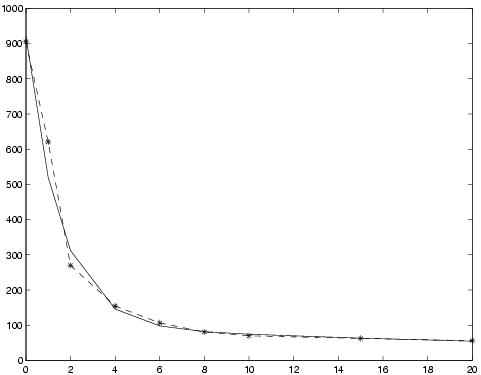
|
|
| ti |
0 |
1.00 |
2.00 |
4.00 |
6.00 |
8.00 |
10.00 |
15.00 |
20.00 |
| yi |
905.10 |
620.36 |
270.17 |
154.68 |
106.74 |
80.92 |
69.98 |
62.50 |
56.29 |
|
To set up and solve the problem of fitting the data to a two-term
exponential model
f(t) = α1 e−β1 t + α2 e−β2 t,
give the following commands:
>> p      = 2;                         % Two terms
>> Name   = 'Simple two-term exp fit'; % Problem name, can be anything
>> wType  = 0;                         % No weighting
>> SepAlg = 0;                         % Separable problem
>> Prob = expAssign(p,Name,t,y,wType,[],SepAlg);

>> Result = tomRun('expSolve',Prob,1);
>> x = Result.x_k'

x =
          0.01          0.58         72.38        851.68
The
x vector contains the parameters as
x=[β
1,β
2,α
1,α
2] so the solution may be
visualized with
>> plot(t,y,'-*', t,x(3)*exp(-t*x(1)) + x(4)*exp(-t*x(2)) );
Figure 18: Results of fitting experimental data to two-term exponential model. Solid line: final model, dash-dot: data.
Purpose
Solve box-bounded global optimization problems.
glbDirect solves problems of the form
where
f R and
x,
xL,
xU R n.
glbDirect is a Fortran MEX implementation of
glbSolve .
Calling Syntax
Result = glbDirectTL(Prob,varargin)
Result = tomRun('glbDirect', Prob);
Description of Inputs
| Prob |
Problem description structure. The following fields are used: |
| |
| Prob |
Problem description structure. The following fields are used:, continued |
| |
| |
x_L |
Lower bounds for x, must be given to restrict
the search space. |
| |
x_U |
Upper bounds for x, must be given to restrict
the search space. |
| |
| |
Name |
Name of the problem. Used for security if doing warm start. |
| |
FUNCS.f |
Name of m-file computing the objective function f(x). |
| |
| |
PriLevOpt |
Print Level. 0 = Silent. 1 = Errors. 2 = Termination message and warm start info. 3 = Option summary. |
| |
| |
WarmStart |
If true, >0, glbDirect reads the output
from the last run from Prob.glbDirect.WarmStartInto if it
exists. If it doesn't exist, glbDirect attempts to open and
read warm start data from mat-file glbDirectSave.mat.
glbDirect uses this warm start information to continue from the last run. |
| |
| |
optParam |
Structure in Prob, Prob.optParam. Defines optimization parameters. Fields used: |
| |
| |
IterPrint |
Print iteration log every IterPrint
iteration. Set to 0 for no iteration log. PriLev must be set to at
least 1 to have iteration log to be printed. |
| |
MaxIter |
Maximal number of iterations, default 200. |
| |
MaxFunc |
Maximal number of function evaluations, default 10000 (roughly). |
| |
EpsGlob |
Global/local weight parameter, default 1E-4. |
| |
fGoal |
Goal for function value, if empty not used. |
| |
eps_f |
Relative accuracy for function value, fTol == epsf. Stop if abs(f−fGoal) <= abs(fGoal) * fTol , if fGoal =0. Stop if abs(f−fGoal) <= fTol , if fGoal == 0. |
| |
eps_x |
Convergence tolerance in x. All possible rectangles are less than this tolerance (scaled to (0,1) ). See the output field maxTri. |
| |
| |
glbDirect |
Structure in Prob, Prob.glbDirect. Solver specific. |
| |
options |
Structure with options. These options have
precedence over all other options in the Prob struct. Available
options are: |
| |
| |
|
PRILEV: Equivalent to Prob.PrilevOpt. Default: 0 |
| |
|
MAXFUNC: Eq. to Prob.optParam.MaxFunc. Default: 10000 |
| |
|
MAXITER: Eq. to Prob.optParam.MaxIter. Default: 200 |
| |
|
PARALLEL: Set to 1 in order to have glbDirect to call
Prob.FUNCS.f with a matrix x of points to let the user function
compute function values in parallel. Default: 0 |
| |
|
WARMSTART: Eq. to Prob.WarmStart. Default: 0 |
| |
|
ITERPRINT: Eq. to Prob.optParam.IterPrint. Default: 0 |
| |
|
FUNTOL: Eq. to Prob.optParam.eps_f. Default: 1e-2 |
| |
|
VARTOL: Eq. to Prob.optParam.eps_x. Default: 1e-13 |
| |
|
GLWEIGHT: Eq. to Prob.optParam.EpsGlob. Default: 1e-4 |
| |
| |
WarmStartInfo |
Structure with WarmStartInfo. Use
WarmDefDIRECT.m to define it. |
| |
Description of Outputs
| Result |
Structure
with result from optimization.
The following fields are changed: |
| |
| Result |
Structure
with result from optimization.
The following fields are changed:, continued |
| |
| |
x_k |
Matrix with optimal points as columns. |
| |
f_k |
Function value at optimum. |
| |
| |
Iter |
Number of iterations. |
| |
FuncEv |
Number function evaluations. |
| |
ExitText |
Text string giving ExitFlag and Inform information. |
| |
ExitFlag |
Exit code. |
| |
|
0 = Normal termination, max number of iterations /func.evals reached. |
| |
|
1 = Some bound, lower or upper is missing. |
| |
|
2 = Some bound is inf, must be finite. |
| |
|
4 = Numerical trouble determining optimal rectangle, empty set and cannot continue. |
| |
Inform |
Inform code. |
| |
|
1 = Function value f is less than fGoal. |
| |
|
2 = Absolute function value f is less than fTol, only if fGoal = 0 or Relative error in function value f is less than fTol, i.e. abs(f−fGoal)/abs(fGoal) <= fTol. |
| |
|
3 = Maximum number of iterations done. |
| |
|
4 = Maximum number of function evaluations done. |
| |
|
91= Numerical trouble, did not find element in list. |
| |
|
92= Numerical trouble, No rectangle to work on. |
| |
|
99= Other error, see ExitFlag. |
| |
| |
glbDirect |
Substructure for glbDirect specific result data. |
| |
| |
nextIterFunc |
If optimization algorithm was stopped
because of maximum number of function evaluations reached, this is
the number of function evaluations required to complete the next
iteration. |
| |
maxTri |
Maximum size of any triangles. |
| |
WarmStartInfo |
Structure containing warm start data.
Could be used to continue optimization where glbDirect stopped. |
| |
| |
To make a warm start possible, glbDirect saves the following information in |
| |
the structure Result.glbDirect.WarmStartInfo and file |
| |
glbDirectSave.mat (for internal solver use only): |
| |
| |
points |
Matrix with all rectangle centerpoints, in [0,1]-space. |
| |
dRect |
Vector with distances from centerpoint to the vertices. |
| |
fPoints |
Vector with function values. |
| |
nIter |
Number of iterations. |
| |
lRect |
Matrix with all rectangle side lengths in each dimension. |
| |
Name |
Name of the problem. Used for security if doing warm start. |
| |
dMin |
Row vector of minimum function value for each distance. |
| |
ds |
Row vector of all different distances, sorted. |
| |
glbfMin |
Best function value found at a feasible point. |
| |
iMin |
The index in D which has lowest function
value, i.e. the rectangle which minimizes (F − glbfMin + E)./D
where E = max(EpsGlob*abs(glbfMin),1E−8). |
| |
ign |
Rectangles to be ignored in the rect. selection procedure. |
| |
Description
The global optimization routine
glbDirect is an
implementation of the DIRECT algorithm presented in
[
16]. The algorithm in
glbDirect is a Fortran MEX
implementation of the algorithm in
glbSolve . DIRECT
is a modification of the standard Lipschitzian approach that
eliminates the need to specify a Lipschitz constant. Since no such
constant is used, there is no natural way of defining convergence
(except when the optimal function value is known). Therefore
glbDirect runs a predefined number of iterations and
considers the best function value found as the optimal one. It is
possible for the user to
restart glbDirect with the
final status of all parameters from the previous run, a so called
warm start. Assume that a run has been made with
glbDirect on a certain problem for 50 iterations. Then a run
of e.g. 40 iterations more should give the same result as if the run
had been using 90 iterations in the first place. To do a warm start
of
glbDirect a flag
Prob.WarmStart should be set to
one and
WarmDefDIRECT run. Then
glbDirect is using
output previously obtained to make the restart. The m-file
glbSolve also includes the subfunction
conhull (in
MEX) which is an implementation of the algorithm GRAHAMHULL
in [
68, page 108] with the modifications proposed on page
109.
conhull is used to identify all points lying on the
convex hull defined by a set of points in the plane.
M-files Used
iniSolve.m ,
endSolve.m
glbSolve.m .
Purpose
Solve box-bounded global optimization problems.
glbFast solves problems of the form
where
f R and
x,
xL,
xU R n.
glbFast is a Fortran MEX implementation of
glbSolve .
Calling Syntax
Result = glbFast(Prob,varargin)
Result = tomRun('glbFast', Prob);
Description of Inputs
| Prob |
Problem description structure. The following fields are used: |
| |
| Prob |
Problem description structure. The following fields are used:, continued |
| |
| |
x_L |
Lower bounds for x, must be given to restrict
the search space. |
| |
x_U |
Upper bounds for x, must be given to restrict
the search space. |
| |
| |
Name |
Name of the problem. Used for security if doing warm start. |
| |
FUNCS.f |
Name of m-file computing the objective function f(x). |
| |
| |
PriLevOpt |
Print Level. 0 = silent. 1 = Warm Start info 2 = A header printed. |
| |
| |
WarmStart |
If true, >0, glbFast reads the output from the last run from the mat-file glbFastSave.mat, and continues from the last run.. |
| |
| |
optParam |
Structure in Prob, Prob.optParam. Defines optimization parameters. Fields used: |
| |
| |
IterPrint |
Print iteration #, # of evaluated points and best f(x) each iteration. |
| |
MaxIter |
Maximal number of iterations, default max(5000,n*1000). |
| |
MaxFunc |
Maximal number of function evaluations, default max(10000,n*2000). |
| |
EpsGlob |
Global/local weight parameter, default 1E-4. |
| |
fGoal |
Goal for function value, if empty not used. |
| |
eps_f |
Relative accuracy for function value, fTol == epsf. Stop if abs(f−fGoal) <= abs(fGoal) * fTol , if fGoal =0. Stop if abs(f−fGoal) <= fTol , if fGoal == 0. |
| |
eps_x |
Convergence tolerance in x. All possible rectangles are less than this tolerance (scaled to (0,1) ). See the output field maxTri. |
| |
| |
If restart is chosen, the
following fields in glbFastSave.mat are also used |
| |
and contains information from the previous run (for internal solver use only). |
| |
| |
C |
Matrix with all rectangle centerpoints, in [0,1]-space. |
| |
D |
Vector with distances from centerpoint to the vertices. |
| |
E |
Computed tolerance in rectangle selection. |
| |
F |
Vector with function values. |
| |
Iter |
Number of iterations. |
| |
L |
Matrix with all rectangle side lengths in each dimension. |
| |
Name |
Name of the problem. Used for security if doing warm start. |
| |
dMin |
Row vector of minimum function value for each distance. |
| |
ds |
Row vector of all different distances, sorted. |
| |
glbfMin |
Best function value found at a feasible point. |
| |
iMin |
The index in D which has lowest function value, i.e. the rectangle which minimizes (F − glbfMin + E)./D where E = max(EpsGlob*abs(glbfMin),1E−8). |
| |
ignoreIdx |
Rectangles to be ignored in the rect. selection procedure. |
| |
| varargin |
Other parameters directly sent to low level routines. |
Description of Outputs
| Result |
Structure
with result from optimization.
The following fields are changed: |
| |
| Result |
Structure
with result from optimization.
The following fields are changed:, continued |
| |
| |
x_k |
Matrix with all points giving the function value f_k. |
| |
f_k |
Function value at optimum. |
| |
| |
Iter |
Number of iterations. |
| |
FuncEv |
Number function evaluations. |
| |
maxTri |
Maximum size of any triangle. |
| |
ExitText |
Text string giving ExitFlag and Inform information. |
| |
ExitFlag |
Exit code. |
| |
|
0 = Normal termination, max number of iterations /func.evals reached. |
| |
|
1 = Some bound, lower or upper is missing. |
| |
|
2 = Some bound is inf, must be finite. |
| |
|
4 = Numerical trouble determining optimal rectangle, empty set and cannot continue. |
| |
Inform |
Inform code. |
| |
|
1 = Function value f is less than fGoal. |
| |
|
2 = Absolute function value f is less than fTol, only if fGoal = 0 or Relative error in function value f is less than fTol, i.e. abs(f−fGoal)/abs(fGoal) <= fTol. |
| |
|
3 = Maximum number of iterations done. |
| |
|
4 = Maximum number of function evaluations done. |
| |
|
91= Numerical trouble, did not find element in list. |
| |
|
92= Numerical trouble, No rectangle to work on. |
| |
|
99= Other error, see ExitFlag. |
| |
Solver |
Solver used, 'glbFast'. |
| |
Description
The global optimization routine
glbFast is an implementation
of the DIRECT algorithm presented in [
16]. The
algorithm in
glbFast is a Fortran MEX implementation of the
algorithm in
glbSolve . DIRECT is a modification of
the standard Lipschitzian approach that eliminates the need to
specify a Lipschitz constant. Since no such constant is used, there
is no natural way of defining convergence (except when the optimal
function value is known). Therefore
glbFast runs a predefined
number of iterations and considers the best function value found as
the optimal one. It is possible for the user to
restart
glbFast with the final status of all parameters from the
previous run, a so called
warm start. Assume that a run has
been made with
glbFast on a certain problem for 50
iterations. Then a run of e.g. 40 iterations more should give the
same result as if the run had been using 90 iterations in the first
place. To do a warm start of
glbFast a flag
Prob.WarmStart should be set to one. Then
glbFast is
using output previously written to the file
glbFastSave.mat
to make the restart. The m-file
glbSolve also includes the
subfunction
conhull (in MEX) which is an implementation of
the algorithm GRAHAMHULL in [
68, page 108] with
the modifications proposed on page 109.
conhull is used to
identify all points lying on the convex hull defined by a set of
points in the plane.
M-files Used
iniSolve.m ,
endSolve.m
glbSolve.m .
Purpose
Solve box-bounded global optimization problems.
glbSolve solves problems of the form
where
f R and
x,
xL,
xU R n.
Calling Syntax
Result = glbSolve(Prob,varargin)
Result = tomRun('glbSolve', Prob);
Description of Inputs
| Prob |
Problem description structure. The following fields are used: |
| |
| Prob |
Problem description structure. The following fields are used:, continued |
| |
| |
x_L |
Lower bounds for x, must be given to restrict
the search space. |
| |
x_U |
Upper bounds for x, must be given to restrict
the search space. |
| |
| |
Name |
Name of the problem. Used for security if doing warm start. |
| |
FUNCS.f |
Name of m-file computing the objective function f(x). |
| |
| |
PriLevOpt |
Print Level. 0 = silent. 1 = some printing. 2 = print each iteration. |
| |
| |
WarmStart |
If true, >0, glbSolve reads the output from the last run from the mat-file glbSave.mat, and continues from the last run. |
| |
| |
MaxCPU |
Maximal CPU Time (in seconds) to be used. |
| |
| |
optParam |
Structure in Prob, Prob.optParam. Defines optimization parameters. Fields used: |
| |
| |
IterPrint |
Print iteration #, # of evaluated points and best f(x) each iteration. |
| |
MaxIter |
Maximal number of iterations, default max(5000,n*1000). |
| |
MaxFunc |
Maximal number of function evaluations, default max(10000,n*2000). |
| |
EpsGlob |
Global/local weight parameter, default 1E-4. |
| |
fGoal |
Goal for function value, if empty not used. |
| |
eps_f |
Relative accuracy for function value, fTol == epsf. Stop if abs(f−fGoal) <= abs(fGoal) * fTol , if fGoal =0. Stop if abs(f−fGoal) <= fTol , if fGoal == 0. |
| |
| |
If warm start is chosen, the
following fields saved to glbSave.mat are also used |
| |
and contains information from the previous run: |
| |
| |
C |
Matrix with all rectangle centerpoints, in [0,1]-space. |
| |
D |
Vector with distances from centerpoint to the vertices. |
| |
DMin |
Row vector of minimum function value for each distance. |
| |
DSort |
Row vector of all different distances, sorted. |
| |
E |
Computed tolerance in rectangle selection. |
| |
F |
Vector with function values. |
| |
L |
Matrix with all rectangle side lengths in each dimension. |
| |
Name |
Name of the problem. Used for security if doing warm start. |
| |
glbfMin |
Best function value found at a feasible point. |
| |
iMin |
The index in D which has lowest function value, i.e. the rectangle which minimizes (F − glbfMin + E)./D where E = max(EpsGlob*abs(glbfMin),1E−8). |
| |
| varargin |
Other parameters directly sent to low level routines. |
Description of Outputs
| Result |
Structure
with result from optimization.
The following fields are changed: |
| |
| Result |
Structure
with result from optimization.
The following fields are changed:, continued |
| |
| |
x_k |
Matrix with all points giving the function value f_k. |
| |
f_k |
Function value at optimum. |
| |
| |
Iter |
Number of iterations. |
| |
FuncEv |
Number function evaluations. |
| |
maxTri |
Maximum size of any triangle. |
| |
ExitText |
Text string giving ExitFlag and Inform information. |
| |
ExitFlag |
Exit code. |
| |
|
0 = Normal termination, max number of iterations /func.evals reached. |
| |
|
1 = Some bound, lower or upper is missing. |
| |
|
2 = Some bound is inf, must be finite. |
| |
|
4 = Numerical trouble determining optimal rectangle, empty set and cannot continue. |
| |
Inform |
Inform code. |
| |
|
0 = Normal Exit. |
| |
|
1 = Function value f is less than fGoal. |
| |
|
2 = Absolute function value f is less than fTol, only if fGoal = 0 or Relative error in function value f is less than fTol, i.e. abs(f−fGoal)/abs(fGoal) <= fTol. |
| |
|
9 = Max CPU Time reached. |
| |
Solver |
Solver used, 'glbSolve'. |
| |
Description
The global optimization routine
glbSolve is an
implementation of the DIRECT algorithm presented in
[
16]. DIRECT is a modification of the standard
Lipschitzian approach that eliminates the need to specify a
Lipschitz constant. Since no such constant is used, there is no
natural way of defining convergence (except when the optimal
function value is known). Therefore
glbSolve runs a
predefined number of iterations and considers the best function
value found as the optimal one. It is possible for the user to
restart glbSolve with the final status of all
parameters from the previous run, a so called
warm start
Assume that a run has been made with
glbSolve on a certain
problem for 50 iterations. Then a run of e.g. 40 iterations more
should give the same result as if the run had been using 90
iterations in the first place. To do a warm start of
glbSolve a flag
Prob.WarmStart should be set to one.
Then
glbSolve is using output previously written to the
file
glbSave.mat to make the restart. The m-file
glbSolve also includes the subfunction
conhull (in
MEX) which is an implementation of the algorithm GRAHAMHULL in [
68, page 108] with the modifications
proposed on page 109.
conhull is used to identify all
points lying on the convex hull defined by a set of points in the
plane.
M-files Used
iniSolve.m ,
endSolve.m
Purpose
Solve general constrained mixed-integer global optimization
problems using a hybrid algorithm.
glcCluster solves problems of the form
|
|
|
f(x) |
|
|
|
|
| s/t |
xL |
≤ |
x |
≤ |
xU |
| |
bL |
≤ |
Ax |
≤ |
bU |
| |
cL |
≤ |
c(x) |
≤ |
cU |
| |
|
|
xi N i I |
|
where
x,
xL,
xU Rn,
c(
x),
cL,
cU Rm1,
A Rm2× n and
bL,
bU Rm2.
The variables
x I, the index subset of 1,...,
n are
restricted to be integers.
Calling Syntax
Result = glcCluster(Prob, maxFunc1, maxFunc2, maxFunc3, ProbL)
Result = tomRun('glcCluster', Prob, PriLev) (driver call)
Description of Inputs
| Prob |
Problem description structure. The following fields are used: |
| |
| Prob |
Problem description structure. The following fields are used:, continued |
| |
| |
A |
Constraint matrix for linear constraints. |
| |
b_L |
Lower bounds on the linear constraints. |
| |
b_U |
Upper bounds on the linear constraints. |
| |
| |
c_L |
Lower bounds on the general constraints. |
| |
c_U |
Upper bounds on the general constraints. |
| |
| |
x_L |
Lower bounds for x, must be given to restrict the search space. |
| |
x_U |
Upper bounds for x, must be given to restrict the search space. |
| |
| |
FUNCS.f |
Name of m-file computing the objective function f(x). |
| |
FUNCS.c |
Name of m-file computing the vector of constraint functions c(x). |
| |
| |
PriLevOpt |
Print level. 0=Silent. 1=Some output from
each glcCluster phase. 2=More output from each phase. 3=Further
minor output from each phase. 6=Use PrintResult( ,1) to print
summary from each global and local run. 7 = Use PrintResult( ,2)
to print summary from each global and local run. 8 = Use
PrintResult( ,3) to print summary from each global and local run. |
| |
| |
WarmStart |
If true, >0, glcCluster warm starts the
DIRECT solver. The DIRECT solver will utilize all points sampled
in last run, from one or two calls, dependent on the success in
last run. Note: The DIRECT solver may not be changed if doing
WarmStart mat-file glcFastSave.mat, and continues from the last run. |
| |
| |
Name |
Name of the problem. glcCluster uses the
warmstart capability in glcFast and needs the name for
security reasons. |
| |
| |
GO |
Structure in Prob , Prob.GO . Fields used: |
| |
maxFunc1 |
Number of function evaluations in 1st call
to glcFast. Should be odd number (automatically corrected). Default 100*dim(x) + 1. |
| |
maxFunc2 |
Number of function evaluations in 2nd call
to glcFast. |
| |
maxFunc3 |
If glcFast is not feasible after maxFunc1
function evaluations, it will be repeatedly called (warm start)
doing maxFunc1 function evaluations until maxFunc3 function
evaluations reached. |
| |
ProbL |
Structure to be used in the local search. By
default the same problem structure as in the global search is used,
Prob (see below). Using a second structure is important if optimal
continuous variables may take values on bounds. glcFast used for the
global search only converges to the simple bounds in the limit, and
therefore the simple bounds may be relaxed a bit in the global
search. Also, if the global search has difficulty fulfilling
equality constraints exactly, the lower and upper bounds may be
slightly relaxed. But being exact in the local search. Note that the
local search is using derivatives, and can utilize given analytic
derivatives. Otherwise the local solver is using numerical
derivatives or automatic differentiation. If routines to provide
derivatives are given in ProbL, they are used. If only one structure
Prob is given, glcCluster uses the derivative routines given in the
this structure. |
| |
localSolver |
Optionally change local solver used ('snopt' or 'npsol' etc.). |
| |
| |
DIRECT |
DIRECT subsolver, either glcSolve or glcFast (default). |
| |
| |
localTry |
Maximal number of local searches from
cluster points. If <= 0, glcCluster stops after clustering. Default 100. |
| |
| |
maxDistmin |
The minimal number used for clustering, default 0.05. |
| |
| |
optParam |
Structure with special fields for optimization parameters, see Table A. |
| |
|
Fields used are: PriLev , cTol , IterPrint , MaxIter , MaxFunc , |
| |
|
EpsGlob , fGoal , eps_f , eps_x . |
| |
| |
MIP.IntVars |
Structure in Prob, Prob.MIP. If empty, all
variables are assumed non-integer (LP problem). If length(IntVars)
>1 ==> length(IntVars) == length(c) should hold. Then IntVars(i)
==1 ==> x(i) integer. IntVars(i) ==0 ==> x(i) real. If
length(IntVars) < n, IntVars is assumed to be a set of indices. It
is advised to number the integer values as the first variables,
before the continuous. The tree search will then be done
more efficiently. |
| |
| varargin |
Other parameters directly sent to low level routines. |
Description of Outputs
| Result |
Structure
with result from optimization.
The following fields are changed: |
| |
| Result |
Structure
with result from optimization.
The following fields are changed:, continued |
| |
| |
x_k |
Matrix with all points giving the function value f_k. |
| |
f_k |
Function value at optimum. |
| |
c_k |
Nonlinear constraints values at x_k. |
| |
| |
Iter |
Number of iterations. |
| |
FuncEv |
Number function evaluations. |
| |
maxTri |
Maximum size of any triangle. |
| |
ExitText |
Text string giving ExitFlag and Inform information. |
| |
| |
Cluster |
Subfield with clustering information |
| |
x_k |
Matrix with best cluster points. |
| |
f_k |
Row vector with f(x) values for each column in Cluster.x_k. |
| |
maxDist |
maxDist used for clustering. |
| |
minDist |
vector of all minimal distances between points. |
| |
Description
The routine
glcCluster implements an extended version of
DIRECT, see [
55], that handles problems with both
nonlinear and integer constraints.
DIRECT is a modification of the standard Lipschitzian
approach that eliminates the need to specify a Lipschitz constant.
Since no such constant is used, there is no natural way of
defining convergence (except when the optimal function value is
known). Therefore
glcCluster is run for a predefined number
of function evaluations and considers the best function value
found as the optimal one. It is possible for the user to
restart glcCluster with the final status of all parameters
from the previous run, a so called
warm start Assume that a
run has been made with
glcCluster on a certain problem for
500 function evaluations. Then a run of e.g. 200 function
evaluations more should give the same result as if the run had
been using 700 function evaluations in the first place. To do a
warm start of
glcCluster a flag
Prob.WarmStart
should be set to one. Then
glcCluster is using output
previously written to the file
glcSave.mat to make the
restart.
DIRECT does not explicitly handle equality constraints. It works best
when the integer variables describe an ordered quantity and is less effective
when they are categorical.
M-files Used
iniSolve.m ,
endSolve.m ,
glcFast.m
Purpose
Solve global mixed-integer nonlinear programming problems.
glcDirect solves problems of the form
|
|
|
f(x) |
|
|
|
|
| s/t |
xL |
≤ |
x |
≤ |
xU |
| |
bL |
≤ |
Ax |
≤ |
bU |
| |
cL |
≤ |
c(x) |
≤ |
cU |
| |
|
|
xi integer |
|
i I |
|
where
x,
xL,
xU Rn,
c(
x),
cL,
cU Rm1,
A Rm2× n and
bL,
bU Rm2.
The variables
x I, the index subset of 1,...,
n are
restricted to be integers. Recommendation: Put the integers as the
first variables. Put low range integers before large range integers.
Linear constraints are specially treated. Equality constraints are
added as penalties to the objective. Weights are computed
automatically, assuming f(x) scaled to be roughly 1 at optimum.
Otherwise scale f(x).
glcDirect is a Fortran MEX implementation of
glcSolve .
Calling Syntax
Result = glcDirectTL(Prob,varargin)
Result = tomRun('glcDirect', Prob);
Description of Inputs
| Prob |
Problem description structure. The following fields are used: |
| |
| Prob |
Problem description structure. The following fields are used:, continued |
| |
| |
Name |
Problem name. Used for safety when doing warm starts. |
| |
| |
FUNCS.f |
Name of m-file computing the objective function f(x). |
| |
FUNCS.c |
Name of m-file computing the vector of constraint functions c(x). |
| |
| |
A |
Linear constraints matrix. |
| |
b_L |
Lower bounds on the linear constraints. |
| |
b_U |
Upper bounds on the linear constraints. |
| |
| |
c_L |
Lower bounds on the general constraints. |
| |
c_U |
Upper bounds on the general constraints. |
| |
x_L |
Lower bounds for x, must be finite to restrict the search space. |
| |
x_U |
Upper bounds for x, must be finite to restrict the search space. |
| |
| |
PriLevOpt |
Print Level. This controls both regular printing
from glcDirect and the amount of iteration log information to print. |
| |
|
0 = Silent. 1 = Warnings and errors printed. Iteration log on
iterations improving function value. 2 = Iteration log on all
iterations. 3 = Log for
each function evaluation. 4 = Print list of parameter settings. |
| |
|
See optParam.IterPrint for more information on iteration log
printing. |
| |
| |
WarmStart |
If true, >0, glcDirect reads the output from
the last run from Prob.glcDirect.WarmStartInfo if it exists. If it
doesn't exist, glcDirect attempts to open and read warm start data
from mat-file glcDirectSave.mat. glcDirect uses this warm start
information to continue from the last run. |
| |
| |
MaxCPU |
Maximum CPU Time (in seconds) to be used. |
| |
| |
MIP |
Structure in Prob , Prob.MIP . |
| |
Intvars |
If empty, all variables are assumed
non-integer (LP problem)
If length(IntVars) >1 ==> length(IntVars) == length(c) should hold
Then IntVars(i) ==1 ==> x(i) integer. IntVars(i) ==0 ==> x(i) real
If length(IntVars) < n, IntVars is assumed to be a set of indices. It is advised to number the integer values as the first
variables, before the continuous. The tree search will then
be done more efficiently. |
| |
| |
fIP |
An upper bound on the optimal f(x) value. If empty, set as Inf. |
| |
| |
xIP |
The x-values giving the fIP value. If fIP empty and xIP given, fIP will be computed if xIP nonempty, its feasibility is checked |
| |
| |
glcDirect |
Structure with DIRECT algorithm specific parameters. Fields used: |
| |
| |
fcALL |
=0 (Default). If linear constraints cannot be
feasible anywhere inside rectangle, skip f(x) and c(x) computation for middle point. |
| |
|
=1 Always compute f(x) and c(x), even if linear
constraints are
not feasible anywhere in rectangle. Do not update rates of change
for the constraints. |
| |
|
=2 Always compute f(x) and c(x), even if linear
constraints are
not feasible anywhere in rectangle. Update rates of change
constraints. |
| |
| |
useRoC |
=1 (Default). Use original Rate of Change
(RoC) for constraints to weight the constraint violations in
selecting which rectangle divide. |
| |
|
=0 Avoid RoC, giving equal weights to all
constraint violations.
Suggested if difficulty to find feasible points. For problems
where linear constraints have been added among the nonlinear
(NOT RECOMMENDED; AVOID!!!), then option useRoc=0 has been
successful, whereas useRoC completely fails. |
| |
|
=2 Avoid RoC for linear constraints, giving
weight one to these
constraint violations, whereas the nonlinear constraints use RoC. |
| |
|
=3 Use RoC for nonlinear constraints, but
linear constraints are
not used to determine which rectangle to use. |
| |
| |
BRANCH |
=0 Divide rectangle by selecting the longest
side, if ties use the lowest index. This is the Jones DIRECT paper strategy. |
| |
|
=1 First branch the integer variables,
selecting the variable
with the least splits. If all integer variables are split, split
on the continuous variables as in BRANCH=0. DEFAULT!
Normally much more efficient than =0 for mixed-integer problems. |
| |
|
=2 First branch the integer variables with 1,2
or 3 possible values,
e.g [0,1],[0,2] variables, selecting the variable with least splits.
Then branch the other integer variables, selecting the variable
with the least splits. If all integer variables are split, split
on the continuous variables as in BRANCH=0. |
| |
|
=3 Like =2, but use priorities on the
variables, similar to
mipSolve , see Prob.MIP.VarWeight. |
| |
| |
RECTIE |
When minimizing the measure to find which new
rectangle to try to
get feasible, there are often ties, several rectangles have the same
minimum. RECTIE = 0 or 1 seems reasonable choices. Rectangles with low
index are often larger then the rectangles with higher index.
Selecting one of each type could help, but often =0 is fastest. |
| |
|
=0 Use the rectangle with value a, with lowest index (original). |
| |
|
=1 (Default): Use 1 of the smallest and 1 of largest rectangles. |
| |
|
=2 Use the last rectangle with the same value a, not the 1st. |
| |
|
=3 Use one of the smallest rectangles with same value a. |
| |
|
=4 Use all rectangles with the same value a, not just the 1st. |
| |
| |
EqConFac |
Weight factor for equality constraints when
adding to objective
function f(x) (Default value 10). The weight is computed as
EqConFac/"right or left hand side constant value", e.g. if
the constraint is Ax <= b, the weight is EqConFac/b
If DIRECT just is pushing down the f(x) value instead of
fulfilling the equality constraints, increase EqConFac. |
| |
| |
AxFeas |
Set nonzero to make glcDirect skip f(x)
evaluations, when the
linear constraints are infeasible, and still no feasible point
has been found. The default is 0. Value 1 demands fcALL == 0.
This option could save some time if f(x) is a bit costly, however
overall performance could on some problems be dramatically worse. |
| |
| |
fEqual |
All points with function values within
tolerance fEqual are considered to be global minima and returned. Default 1E-10. |
| |
| |
LinWeight |
RateOfChange = LinWeight*||a(i,:)|| for
linear constraints. Balance between linear and nonlinear
constraints. Default 0.1. The higher value, the less influence from linear constraints. |
| |
| |
alpha |
Exponential forgetting factor in RoC computation, default 0.9. |
| |
| |
AvIter |
How many values to use in startup of RoC
computation before switching to exponential smoothing with
forgetting factor alpha. Default 50. |
| |
| |
optParam |
Structure with special fields for optimization parameters,
see Table A. |
| |
|
Fields used by glcDirect are: IterPrint ,
bTol , cTol , MaxIter , MaxFunc ,
EpsGlob , fGoal , eps_f , eps_x . |
| |
| varargin |
Other parameters directly sent to low level routines. |
Description of Outputs
| Result |
Structure
with result from optimization.
The following fields are changed: |
| |
| Result |
Structure
with result from optimization.
The following fields are changed:, continued |
| |
| |
x_k |
Matrix with all points giving the function value f_k. |
| |
f_k |
Function value at optimum. |
| |
c_k |
Nonlinear constraints values at x_k. |
| |
| |
Iter |
Number of iterations. |
| |
FuncEv |
Number function evaluations. |
| |
maxTri |
Maximum size of any triangle. |
| |
ExitText |
Text string giving ExitFlag and Inform information. |
| |
ExitFlag |
0 = Normal termination, max number of iterations func.evals reached. |
| |
|
2 = Some upper bounds below lower bounds. |
| |
|
4 = Numerical trouble, and cannot continue. |
| |
|
7 = Reached maxFunc or maxIter, NOT feasible. |
| |
|
8 = Empty domain for integer variables. |
| |
|
10= Input errors. |
| |
| |
Inform |
1 = Function value f is less than fGoal. |
| |
|
2 = Absolute function value f is less than
fTol, only if fGoal = 0 or Relative error in function value f is
less than fTol, i.e.
abs(f-fGoal)/abs(fGoal) <= fTol. |
| |
|
3 = Maximum number of iterations done. |
| |
|
4 = Maximum number of function evaluations done. |
| |
|
5 = Maximum number of function evaluations
would most likely be too many in the next iteration, save warm start
info, stop. |
| |
|
6 = Maximum number of function
evaluations would most likely be too many in the next iteration,
because 2*sLen >= maxFDim - nFunc, save warm start
info, stop. |
| |
|
7 = Space is dense. |
| |
|
8 = Either space is dense, or MIP is dense. |
| |
|
10= No progress in this run, return solution from previous one. |
| |
|
91= Infeasible. |
| |
|
92= No rectangles to work on. |
| |
|
93= sLen = 0, no feasible integer solution exists. |
| |
|
94= All variables are fixed. |
| |
|
95= There exist free constraints. |
| |
| |
glcDirect |
Substructure for glcDirect specific result data. |
| |
| |
convFlag |
Converge status flag from solver. |
| |
WarmStartInfo |
Structure with warm start information.
Use WarmDefDIRECT to reuse this information in another run. |
| |
| |
glcDirectSave.mat |
To make a warm start possible, glcDirect
saves the following information in the structure
Result.glcDirect.WarmStartInfo and file glcDirectSave.mat (for
internal solver use only): |
| |
| |
C |
Matrix with all rectangle centerpoints, in [0,1]-space. |
| |
D |
Vector with distances from centerpoint to the vertices. |
| |
F |
Vector with function values. |
| |
G |
Matrix with constraint values for each point. |
| |
Iter |
Number of iterations. |
| |
Name |
Name of the problem. Used for security if doing warm start. |
| |
Split |
Split(i,j) is the number of splits along
dimension i of rectangle j. |
| |
Tr |
Tr(i) is the number of times rectangle i
has been trisected. |
| |
fMinIdx |
Indices of the currently best points. |
| |
fMinEQ |
sum(abs(infeasibilities)) for minimum points, 0 if no equalities. |
| |
glcfMin |
Best function value found at a feasible point. |
| |
feasible |
Flag indicating if a feasible point has been found. |
| |
ignoreidx |
Rectangles to be ignored in the rectangle
selection procedure. |
| |
roc |
Rate of change s, for each constraint. |
| |
s0 |
Sum of observed rate of change s0 in the objective. |
| |
t |
t(i) is the total number of splits along
dimension i. |
| |
Description
The routine
glcDirect implements an extended version of
DIRECT, see [
55], that handles problems with both
nonlinear and integer constraints. The algorithm in
glcDirect
is a Fortran MEX implementation of the algorithm in
glcSolve .
DIRECT is a modification of the standard Lipschitzian
approach that eliminates the need to specify a Lipschitz constant.
Since no such constant is used, there is no natural way of defining
convergence (except when the optimal function value is known).
Therefore
glcDirect is run for a predefined number of
function evaluations and considers the best function value found as
the optimal one. It is possible for the user to
restart
glcDirect with the final status of all parameters from the
previous run, a so called
warm start. Assume that a run has
been made with
glcDirect on a certain problem for 500
function evaluations. Then a run of e.g. 200 function evaluations
more should give the same result as if the run had been using 700
function evaluations in the first place. To do a warm start of
glcDirect a flag
Prob.WarmStart should be set to one.
Then
glcDirect will use output previously written to the file
glcDirectSave.mat (or the warm start structure) to make the
restart.
DIRECT does not explicitly handle equality constraints. It
works best when the integer variables describe an ordered quantity
and is less effective when they are categorical.
M-files Used
iniSolve.m ,
endSolve.m and
glcSolve.m .
Warnings
A significant portion of
glcDirect is coded in Fortran MEX format. If the solver is aborted, it may have allocated
memory for the computations which is not returned. This may lead to unpredictable behavior if
glcDirect is started again.
To reduce the risk of trouble, do “
clear mex” if a run has been aborted.
Purpose
Solve global mixed-integer nonlinear programming problems.
glcFast solves problems of the form
|
|
|
f(x) |
|
|
|
|
| s/t |
xL |
≤ |
x |
≤ |
xU |
| |
bL |
≤ |
Ax |
≤ |
bU |
| |
cL |
≤ |
c(x) |
≤ |
cU |
| |
|
|
xi integer |
|
i I |
|
where
x,
xL,
xU Rn,
c(
x),
cL,
cU Rm1,
A Rm2× n and
bL,
bU Rm2.
The variables
x I, the index subset of 1,...,
n are
restricted to be integers. Recommendation: Put the integers as the
first variables. Put low range integers before large range integers.
Linear constraints are specially treated. Equality constraints are
added as penalties to the objective. Weights are computed
automatically, assuming f(x) scaled to be roughly 1 at optimum.
Otherwise scale f(x).
glcFast is a Fortran MEX implementation of
glcSolve .
Calling Syntax
Result = glcFast(Prob,varargin)
Result = tomRun('glcFast', Prob);
Description of Inputs
| Prob |
Problem description structure. The following fields are used: |
| |
| Prob |
Problem description structure. The following fields are used:, continued |
| |
| |
A |
Linear constraints matrix. |
| |
b_L |
Lower bounds on the linear constraints. |
| |
b_U |
Upper bounds on the linear constraints. |
| |
| |
c_L |
Lower bounds on the general constraints. |
| |
c_U |
Upper bounds on the general constraints. |
| |
x_L |
Lower bounds for x, must be finite to restrict the search space. |
| |
x_U |
Upper bounds for x, must be finite to restrict the search space. |
| |
| |
MIP |
Structure in Prob , Prob.MIP . |
| |
Intvars |
If empty, all variables are assumed non-integer (LP problem)
If length(IntVars) >1 ==> length(IntVars) == length(c) should hold
Then IntVars(i) ==1 ==> x(i) integer. IntVars(i) ==0 ==> x(i) real
If length(IntVars) < n, IntVars is assumed to be a set of indices. It is advised to number the integer values as the first
variables, before the continuous. The tree search will then
be done more efficiently. |
| |
| |
fIP |
An upper bound on the optimal f(x) value. If empty, set as Inf. |
| |
| |
xIP |
The x-values giving the fIP value. If fIP empty and xIP given, fIP will be computed if xIP nonempty, its feasibility is checked |
| |
| |
FUNCS.f |
Name of m-file computing the objective function f(x). |
| |
FUNCS.c |
Name of m-file computing the vector of constraint functions c(x). |
| |
| |
Name |
Problem name. Used for safety when doing warm starts. |
| |
| |
WarmStart |
Set to 1 makes glcFast read data from glcFastSave.mat and resume optimization from where previous run ended. See below for details. |
| |
| |
If WarmStart is chosen, the
following fields in glcFastSave.mat are also used |
| |
and contains information from the previous run: |
| |
C |
Matrix with all rectangle centerpoints. |
| |
D |
Vector with distances from centerpoint to the vertices. |
| |
F |
Vector with function values. |
| |
G |
Matrix with constraint values for each point. |
| |
Iter |
Number of iterations. |
| |
Name |
Name of the problem. Used for security if doing warm start. |
| |
Split |
Split(i,j) is the number of splits along
dimension i of rectangle j. |
| |
Tr |
Tr(i) is the number of times rectangle i
has been trisected. |
| |
fMinIdx |
Indices of the currently best points. |
| |
fMinEQ |
sum(abs(infeasibilities)) for minimum points, 0 if no equalities. |
| |
glcfMin |
Best function value found at a feasible point. |
| |
feasible |
Flag indicating if a feasible point has been found. |
| |
ignoreidx |
Rectangles to be ignored in the rectangle
selection procedure. |
| |
roc |
Rate of change s, for each constraint. |
| |
s_0 |
Sum of observed rate of change s0 in the objective. |
| |
t |
t(i) is the total number of splits along
dimension i. |
| |
| |
PriLevOpt |
Print level. 0 = silent. 1 = Warm Start info,
and same output as IterPrint = 1 (see below). 2 = Printing each
iteration, Print iteration number, number of evaluated points, best
f(x) so far and its x-values each iteration, where the best point
has improved. 3 = As PriLevOpt=2, also print sampled x, f(x) and if
feasible. |
| |
| |
MaxCPU |
Maximum CPU Time (in seconds) to be used. |
| |
| |
glcDirect |
Structure with DIRECT algorithm specific parameters. Fields used: |
| |
| |
fcALL |
=0 (Default). If linear constraints cannot be
feasible anywhere inside rectangle, skip f(x) and c(x) computation for middle point. |
| |
|
=1 Always compute f(x) and c(x), even if linear
constraints are
not feasible anywhere in rectangle. Do not update rates of change
for the constraints. |
| |
|
=2 Always compute f(x) and c(x), even if linear
constraints are
not feasible anywhere in rectangle. Update rates of change
constraints. |
| |
| |
AxFeas |
Set nonzero to make glcSolve skip f(x)
evaluations, when the
linear constraints are infeasible, and still no feasible point
has been found. The default is 0. Value 1 demands fcALL == 0.
This option could save some time if f(x) is a bit costly, however
overall performance could on some problems be dramatically worse. |
| |
| |
fEqual |
All points with function values within
tolerance fEqual are considered to be global minima and returned. Default 1E-10. |
| |
| |
LinWeight |
RateOfChange = LinWeight*||a(i,:)|| for
linear constraints. Balance between linear and nonlinear
constraints. Default 0.1. The higher value, the less influence from linear constraints. |
| |
| |
optParam |
Structure with special fields for optimization parameters,
see Table A. |
| |
|
Fields used by glcFast are: IterPrint , bTol ,
cTol , MaxIter (default max(5000,n*1000)),
MaxFunc (default max(10000,n*2000)), EpsGlob ,
fGoal , eps_f ,
eps_x . |
| |
| varargin |
Other parameters directly sent to low level routines. |
Description of Outputs
| Result |
Structure
with result from optimization.
The following fields are changed: |
| |
| Result |
Structure
with result from optimization.
The following fields are changed:, continued |
| |
| |
x_k |
Matrix with all points giving the function value f_k. |
| |
f_k |
Function value at optimum. |
| |
c_k |
Nonlinear constraints values at x_k. |
| |
| |
glcFastSave.mat |
Special file containing: |
| |
| |
C |
Matrix with all rectangle centerpoints. |
| |
D |
Vector with distances from centerpoint to the vertices. |
| |
F |
Vector with function values. |
| |
G |
Matrix with constraint values for each point. |
| |
Iter |
Number of iterations. |
| |
Name |
Name of the problem. Used for security if doing warm start. |
| |
Split |
Split(i,j) is the number of splits along
dimension i of rectangle j. |
| |
Tr |
Tr(i) is the number of times rectangle i
has been trisected. |
| |
fMinIdx |
Indices of the currently best points. |
| |
fMinEQ |
sum(abs(infeasibilities)) for minimum points, 0 if no equalities. |
| |
glcfMin |
Best function value found at a feasible point. |
| |
feasible |
Flag indicating if a feasible point has been found. |
| |
ignoreidx |
Rectangles to be ignored in the rectangle
selection procedure. |
| |
roc |
Rate of change s, for each constraint. |
| |
s_0 |
Sum of observed rate of change s0 in the objective. |
| |
t |
t(i) is the total number of splits along
dimension i. |
| |
| |
Iter |
Number of iterations. |
| |
FuncEv |
Number function evaluations. |
| |
maxTri |
Maximum size of any triangle. |
| |
ExitText |
Text string giving ExitFlag and Inform information. |
| |
ExitFlag |
0 = Normal termination, max number of iterations
/func.evals reached. 2 = Some upper bounds below lower bounds. 4 =
Numerical trouble, and cannot continue. 7 = Reached maxFunc or
maxIter, NOT feasible. 8 = Empty domain for integer variables. |
| |
Inform |
1 = Function value f is less than fGoal. 2 =
Absolute function value f is less than fTol, only if fGoal = 0 or
Relative error in function value f is less than fTol, i.e.
abs(f-fGoal)/abs(fGoal) <= fTol. 3 = Maximum number of iterations
done. 4 = Maximum number of function evaluations done. 5 = Maximum
number of function evaluations would most likely be too many in the
next iteration, save warm start info, stop. 6 = Maximum number of
function evaluations would most likely be too many in the next
iteration, because 2*sLen .GE. maxFDim - nFunc, save warm start
info, stop. 7 = Space is dense. 8 = Either space is dense, or MIP is
dense. 10= No progress in this run, return solution from previous
one. 91= Infeasible. 92= No rectangles to work on. 93= sLen = 0,
no feasible integer solution exists. |
| |
Description
The routine
glcFast implements an extended version of
DIRECT, see [
55], that handles problems with both
nonlinear and integer constraints.
The algorithm in
glcFast is a Fortran MEX implementation of
the algorithm in
glcSolve .
DIRECT is a modification of the standard Lipschitzian
approach that eliminates the need to specify a Lipschitz constant.
Since no such constant is used, there is no natural way of defining
convergence (except when the optimal function value is known).
Therefore
glcFast is run for a predefined number of function
evaluations and considers the best function value found as the
optimal one. It is possible for the user to
restart
glcFast with the final status of all parameters from the
previous run, a so called
warm start. Assume that a run has
been made with
glcFast on a certain problem for 500 function
evaluations. Then a run of e.g. 200 function evaluations more
should give the same result as if the run had been using 700
function evaluations in the first place. To do a warm start of
glcFast a flag
Prob.WarmStart should be set to one.
Then
glcFast will use output previously written to the file
glcFastSave.mat to make the restart.
DIRECT does not explicitly handle equality constraints. It
works best when the integer variables describe an ordered quantity
and is less effective when they are categorical.
M-files Used
iniSolve.m ,
endSolve.m and
glbSolve.m .
Warnings
A significant portion of
glcFast is coded in Fortran MEX format. If the solver is aborted, it may have allocated
memory for the computations which is not returned. This may lead to unpredictable behavior if
glcFast is started again.
To reduce the risk of trouble, do “
clear mex” if a run has been aborted.
Purpose
Solve general constrained mixed-integer global optimization
problems.
glcSolve solves problems of the form
|
|
|
f(x) |
|
|
|
|
| s/t |
xL |
≤ |
x |
≤ |
xU |
| |
bL |
≤ |
Ax |
≤ |
bU |
| |
cL |
≤ |
c(x) |
≤ |
cU |
| |
|
|
xi integer |
|
i I |
|
where
x,
xL,
xU Rn,
c(
x),
cL,
cU Rm1,
A Rm2× n and
bL,
bU Rm2.
The variables
x I, the index subset of 1,...,
n are
restricted to be integers. Recommendation: Put the integers as the
first variables. Put low range integers before large range integers.
Linear constraints are specially treated. Equality constraints are
added as penalties to the objective. Weights are computed
automatically, assuming f(x) scaled to be roughly 1 at optimum.
Otherwise scale f(x).
Calling Syntax
Result = glcSolve(Prob,varargin)
Result = tomRun('glcSolve', Prob);
Description of Inputs
| Prob |
Problem description structure. The following fields are used: |
| |
| Prob |
Problem description structure. The following fields are used:, continued |
| |
| |
A |
Constraint matrix for linear constraints. |
| |
b_L |
Lower bounds on the linear constraints. |
| |
b_U |
Upper bounds on the linear constraints. |
| |
| |
c_L |
Lower bounds on the general constraints. |
| |
c_U |
Upper bounds on the general constraints. |
| |
| |
MIP |
Structure in Prob , Prob.MIP . |
| |
Intvars |
If empty, all variables are assumed non-integer (LP problem)
If length(IntVars) >1 ==> length(IntVars) == length(c) should hold
Then IntVars(i) ==1 ==> x(i) integer. IntVars(i) ==0 ==> x(i) real
If length(IntVars) < n, IntVars is assumed to be a set of indices. It is advised to number the integer values as the first
variables, before the continuous. The tree search will then
be done more efficiently. |
| |
| |
fIP |
An upper bound on the optimal f(x) value. If empty, set as Inf. |
| |
| |
xIP |
The x-values giving the fIP value. If fIP empty and xIP given, fIP will be computed if xIP nonempty, its feasibility is checked |
| |
| |
x_L |
Lower bounds for x, must be given to restrict the search space. Any lower bounds that are inf are changed to -10000. |
| |
x_U |
Upper bounds for x, must be given to restrict the search space. Any upper bounds that are inf are changed to 10000. |
| |
| |
FUNCS.f |
Name of m-file computing the objective function f(x). |
| |
FUNCS.c |
Name of m-file computing the vector of constraint functions c(x). |
| |
| |
Name |
Name of the problem. Used for security if doing warm start. |
| |
| |
PriLevOpt |
Print level. 0 = silent. 1 = some printing. 2 = print each iteration. |
| |
| |
WarmStart |
If true (>0), glcSolve reads the output
from the last run from the mat-file glcSave.mat , and
continues from the last run. NOTE: All rectangles that are fathomed
in the previous run are deleted. This saves space and computational
time and enables solving larger problems and more function evaluations to be done. |
| |
| |
MaxCPU |
Maximal CPU Time (in seconds) to be used. |
| |
| |
glcDirect |
Structure with DIRECT algorithm specific parameters. Fields used: |
| |
| |
fcALL |
=0 (Default). If linear constraints cannot be
feasible anywhere inside rectangle, skip f(x) and c(x) computation for middle point. |
| |
|
=1 Always compute f(x) and c(x), even if linear
constraints are
not feasible anywhere in rectangle. Do not update rates of change
for the constraints. |
| |
|
=2 Always compute f(x) and c(x), even if linear
constraints are
not feasible anywhere in rectangle. Update rates of change
constraints. |
| |
| |
useRoC |
=1 (Default). Use original Rate of Change
(RoC) for constraints to weight the constraint violations in
selecting which rectangle divide. |
| |
|
=0 Avoid RoC, giving equal weights to all
constraint violations.
Suggested if difficulty to find feasible points. For problems
where linear constraints have been added among the nonlinear
(NOT RECOMMENDED; AVOID!!!), then option useRoc=0 has been
successful, whereas useRoC completely fails. |
| |
|
=2 Avoid RoC for linear constraints, giving
weight one to these
constraint violations, whereas the nonlinear constraints use RoC. |
| |
|
=3 Use RoC for nonlinear constraints, but
linear constraints are
not used to determine which rectangle to use. |
| |
| |
BRANCH |
=0 Divide rectangle by selecting the longest
side, if ties use the lowest index. This is the Jones DIRECT paper strategy. |
| |
|
=1 First branch the integer variables,
selecting the variable
with the least splits. If all integer variables are split, split
on the continuous variables as in BRANCH=0. DEFAULT!
Normally much more efficient than =0 for mixed-integer problems. |
| |
|
=2 First branch the integer variables with 1,2
or 3 possible values,
e.g [0,1],[0,2] variables, selecting the variable with least splits.
Then branch the other integer variables, selecting the variable
with the least splits. If all integer variables are split, split
on the continuous variables as in BRANCH=0. |
| |
|
=3 Like =2, but use priorities on the
variables, similar to
mipSolve , see Prob.MIP.VarWeight. |
| |
| |
RECTIE |
When minimizing the measure to find which new
rectangle to try to
get feasible, there are often ties, several rectangles have the same
minimum. RECTIE = 0 or 1 seems reasonable choices. Rectangles with low
index are often larger then the rectangles with higher index.
Selecting one of each type could help, but often =0 is fastest. |
| |
|
=0 Use the rectangle with value a, with lowest index (original). |
| |
|
=1 (Default): Use 1 of the smallest and 1 of largest rectangles. |
| |
|
=2 Use the last rectangle with the same value a, not the 1st. |
| |
|
=3 Use one of the smallest rectangles with same value a. |
| |
|
=4 Use all rectangles with the same value a, not just the 1st. |
| |
| |
EqConFac |
Weight factor for equality constraints when
adding to objective
function f(x) (Default value 10). The weight is computed as
EqConFac/"right or left hand side constant value", e.g. if
the constraint is Ax <= b, the weight is EqConFac/b
If DIRECT just is pushing down the f(x) value instead of
fulfilling the equality constraints, increase EqConFac. |
| |
| |
AxFeas |
Set nonzero to make glcSolve skip f(x)
evaluations, when the
linear constraints are infeasible, and still no feasible point
has been found. The default is 0. Value 1 demands fcALL == 0.
This option could save some time if f(x) is a bit costly, however
overall performance could on some problems be dramatically worse. |
| |
| |
fEqual |
All points with function values within
tolerance fEqual are considered to be global minima and returned. Default 1E-10. |
| |
| |
LinWeight |
RateOfChange = LinWeight*||a(i,:)|| for
linear constraints. Balance between linear and nonlinear
constraints. Default 0.1. The higher value, the less influence from linear constraints. |
| |
| |
alpha |
Exponential forgetting factor in RoC computation, default 0.9. |
| |
| |
AvIter |
How many values to use in startup of RoC
computation before switching to exponential smoothing with
forgetting factor alpha. Default 50. |
| |
| |
If WarmStart is chosen, the
following fields in glcSave.mat are also used |
| |
and contains information from the previous run: |
| |
| |
C |
Matrix with all rectangle centerpoints. |
| |
D |
Vector with distances from centerpoint to the vertices. |
| |
F |
Vector with function values. |
| |
G |
Matrix with constraint values for each point. |
| |
Name |
Name of the problem. Used for security if doing warm start. |
| |
Split |
Split(i,j) is the number of splits along
dimension i of rectangle j. |
| |
T |
T(i) is the number of times rectangle i
has been trisected. |
| |
fMinEQ |
sum(abs(infeasibilities)) for minimum points, 0 if no equalities. |
| |
fMinIdx |
Indices of the currently best points. |
| |
feasible |
Flag indicating if a feasible point has been found. |
| |
glcfmin |
Best function value found at a feasible point. |
| |
iL |
iL(i,j) is the lower bound for rectangle
j in integer dimension I(i). |
| |
iU |
iU(i,j) is the upper bound for rectangle
j in integer dimension I(i). |
| |
ignoreidx |
Rectangles to be ignored in the rectangle
selection procedure. |
| |
s |
s(j) is the sum of observed rates of
change for constraint j. |
| |
s_0 |
s_0 is used as s(0). |
| |
t |
t(i) is the total number of splits along
dimension i. |
| |
SubRes |
Additional output from nlp_f, if suboptimization done. |
| |
| |
optParam |
Structure with special fields for optimization parameters,
see Table A. |
| |
|
Fields used by glcSolve are: IterPrint , bTol ,
cTol , MaxIter (default max(5000,n*1000)),
MaxFunc (default max(10000,n*2000)),
EpsGlob , fGoal , eps_f , eps_x . |
| |
| varargin |
Other parameters directly sent to low level routines. |
Description of Outputs
| Result |
Structure
with result from optimization.
The following fields are changed: |
| |
| Result |
Structure
with result from optimization.
The following fields are changed:, continued |
| |
| |
x_k |
Matrix with all points giving the function value f_k. |
| |
f_k |
Function value at optimum. |
| |
c_k |
Nonlinear constraints values at x_k. |
| |
| |
glcSave.mat |
Special file containing: |
| |
| |
C |
Matrix with all rectangle centerpoints. |
| |
D |
Vector with distances from centerpoint to the vertices. |
| |
F |
Vector with function values. |
| |
G |
Matrix with constraint values for each point. |
| |
Name |
Name of the problem. Used for security if doing warm start. |
| |
Split |
Split(i,j) is the number of splits along
dimension i of rectangle j. |
| |
T |
T(i) is the number of times rectangle i
has been trisected. |
| |
fMinEQ |
sum(abs(infeasibilities)) for minimum points, 0 if no equalities. |
| |
fMinIdx |
Indices of the currently best points. |
| |
feasible |
Flag indicating if a feasible point has been found. |
| |
glcf_min |
Best function value found at a feasible point. |
| |
iL |
iL(i,j) is the lower bound for rectangle
j in integer dimension I(i). |
| |
iU |
iU(i,j) is the upper bound for rectangle
j in integer dimension I(i). |
| |
ignoreidx |
Rectangles to be ignored in the rectangle
selection procedure. |
| |
s |
s(j) is the sum of observed rates of
change for constraint j. |
| |
s_0 |
s_0 is used as s(0). |
| |
t |
t(i) is the total number of splits along
dimension i. |
| |
| |
Iter |
Number of iterations. |
| |
FuncEv |
Number function evaluations. |
| |
maxTri |
Maximum size of any triangle. |
| |
ExitText |
Text string giving ExitFlag and Inform information. |
| |
ExitFlag |
0 - Reached maxFunc or maxIter. 2 - Some upper bounds below lower bounds. 7 - Reached maxFunc or maxIter, NOT feasible. 8 - Empty domain for integer variables. |
| |
Inform |
1 = Function value f is less than fGoal. 2 = Absolute function value f is less than fTol, only if fGoal = 0 or Relative error in function value f is less than fTol, i.e. abs(f-fGoal)/abs(fGoal) <= fTol. 3 = Maximum number of iterations done. 4 = Maximum number of function evaluations done. 9 = Max CPU Time reached. 91= Infeasible. 99= Input error, see ExitFlag. |
| |
Description
The routine
glcSolve implements an extended version of
DIRECT, see [
55], that handles problems with both
nonlinear and integer constraints.
DIRECT is a modification of the standard Lipschitzian
approach that eliminates the need to specify a Lipschitz constant.
Since no such constant is used, there is no natural way of defining
convergence (except when the optimal function value is known).
Therefore
glcSolve is run for a predefined number of function
evaluations and considers the best function value found as the
optimal one. It is possible for the user to
restart
glcSolve with the final status of all parameters from the
previous run, a so called
warm start Assume that a run has
been made with
glcSolve on a certain problem for 500 function
evaluations. Then a run of e.g. 200 function evaluations more
should give the same result as if the run had been using 700
function evaluations in the first place. To do a warm start of
glcSolve a flag
Prob.WarmStart should be set to one.
Then
glcSolve is using output previously written to the file
glcSave.mat to make the restart.
DIRECT does not explicitly handle equality constraints. It
works best when the integer variables describe an ordered quantity
and is less effective when they are categorical.
M-files Used
iniSolve.m ,
endSolve.m
Purpose
Finds a linearly constrained minimax solution of a function of
several variables with the use of any suitable TOMLAB solver. The
decision variables may be binary or integer.
infLinSolve solves problems of the type:
|
|
|
maxDx |
| subject to |
xL |
≤ |
x |
≤ |
xU |
| |
bL |
≤ |
Ax |
≤ |
bU |
|
where
x,
xL,
xU Rn,
bL,
bU Rm1,
A
Rm1 × n and
D Rm2 × n. The variables
x I, the index subset of 1,...,
n are restricted to be
integers. The different objectives are stored in D row-wise.
Calling Syntax
Result=infLinSolve(Prob,PriLev)
Description of Inputs
| Prob |
Structure Prob. Prob must be defined. Best is to use Prob = lp/mipAssign(.....), if using the TQ format. Prob.QP.D matrix should then be set to the rows (Prob.QP.c
ignored). |
| |
| PriLev |
Print level in infLinSolve . |
| |
| =0 |
Silent except for error messages. |
| >0 |
Print summary information about problem transformation. |
| |
Calls PrintResult with specified PriLev . |
| =2 |
Standard output from PrintResult (default). |
|
| |
| |
Extra fields used in Prob: |
| |
| SolverInf |
Name of the TOMLAB solver. Valid names are:
cplex, minos, snopt, xa and more. See SolverList('lp');
or SolverList('mip'); |
| |
| QP.D |
The rows with the different objectives. |
| |
| f_Low |
Lower bound on the objective (optional). |
| |
| f_Upp |
Upper bound on the objective (optional). |
| |
Description of Outputs
| Result |
Structure with results from optimization. Output depends on the solver used. |
| |
| |
The fields x_k , f_k , x_0 , xState , bState , v_k are
transformed back to match the original problem. |
| |
| |
The output in Result.Prob is the result after infLinSolve transformed
the problem, i.e. the altered Prob structure |
Description
The linear minimax problem is solved in infLinSolve by rewriting the problem
as a linear optimization problem. One additional
variable
z R, stored as
xn+1 is added and the
problem is rewritten as:
|
|
|
| |
| subject to |
xL |
≤ |
(x1,x2,…,xn)T |
≤ |
xU |
| |
−∞ |
≤ |
z |
≤ |
∞ |
| |
bL |
≤ |
A x |
≤ |
bU |
| |
−∞ |
≤ |
D x − z e |
≤ |
0 |
|
where
e RN,
e(
i)=1
i.
To handle cases where a row in D*x is taken the absolute value of:
min max |
D*
x|, expand the problem with extra residuals with the
opposite sign: [
D*
x; −
D*
x].
See Also
lpAssign .
Purpose
Find a constrained minimax solution with the use of any suitable
TOMLAB solver.
infSolve solves problems of the type:
|
|
|
maxr(x) |
| subject to |
xL |
≤ |
x |
≤ |
xU |
| |
bL |
≤ |
Ax |
≤ |
bU |
| |
cL |
≤ |
c(x) |
≤ |
cU |
|
where
x,
xL,
xU Rn,
r(
x)
RN,
c(
x),
cL,
cU
Rm1,
bL,
bU Rm2 and
A Rm2 × n.
Calling Syntax
Result=infSolve(Prob,PriLev)
Description of Inputs
| Prob |
Problem description structure. Should be created in the cls format. infSolve uses two special fields in Prob : |
| |
| |
| SolverInf |
Name of solver used to solve the transformed problem. |
| |
Valid choices are conSolve , nlpSolve , sTrustr and clsSolve . |
| |
If TOMLAB /SOL is installed: minos , snopt , npopt . |
| InfType |
1 - constrained formulation (default). |
| |
2 - LS penalty approach (experimental). |
|
| |
The remaining fields of Prob should be defined as required by the selected subsolver. |
| |
| PriLev |
Print level in infSolve . |
| |
| =0 |
Silent except for error messages. |
| >0 |
Print summary information about problem transformation. |
| |
Calls PrintResult with specified PriLev . |
| =2 |
Standard output from PrintResult (default). |
|
Description of Outputs
| Result |
Structure with results from optimization. Output depends on the solver used. |
| |
| |
The fields x_k , r_k , J_k , c_k , cJac , x_0 , xState , cState , v_k are
transformed back to match the original problem. |
| |
| |
g_k is calculated as J_kT r_k . |
| |
| |
The output in Result.Prob is the result after infSolve transformed
the problem, i.e. the altered Prob structure |
Description
The minimax problem is solved in infSolve by rewriting the problem
as a general constrained optimization problem. One additional
variable
z R, stored as
xn+1 is added and the
problem is rewritten as:
|
|
|
| |
| subject to |
xL |
≤ |
(x1,x2,…,xn)T |
≤ |
xU |
| |
−∞ |
≤ |
z |
≤ |
∞ |
| |
bL |
≤ |
A x |
≤ |
bU |
| |
cL |
≤ |
c(x) |
≤ |
cU |
| |
−∞ |
≤ |
r(x) − z e |
≤ |
0 |
|
where
e RN,
e(
i)=1
i.
To handle cases where an element
ri(
x) in
r(
x) appears in absolute
value: minmax|
ri(
x)|, expand the problem with extra residuals
with the opposite sign: [
ri(
x); −
ri(
x) ]
Examples
minimaxDemo.m .
See Also
clsAssign .
Purpose
Finds a linearly constrained solution of a function of the ratio of
two linear functions with the use of any suitable TOMLAB solver.
Binary and integer variables are not supported.
linRatSolve solves problems of the type:
|
|
|
|
| subject to |
xL |
≤ |
x |
≤ |
xU |
| |
bL |
≤ |
Ax |
≤ |
bU |
|
where
c1,
c2,
x,
xL,
xU Rn,
bL,
bU Rm1 and
A Rm1 × n.
Calling Syntax
Result=linRatSolve(Prob,PriLev)
Description of Inputs
| Prob |
Structure Prob. Prob must be defined. Best is to use Prob = lpAssign(.....), if using the TQ format.
Prob.QP.c1/c2 matrices should then be set (Prob.QP.c ignored). |
| |
| PriLev |
Print level in linRatSolve . |
| |
| =0 |
Silent except for error messages. |
| >0 |
Print summary information about problem transformation. |
| |
Calls PrintResult with specified PriLev . |
| =2 |
Standard output from PrintResult (default). |
|
| |
| |
Extra fields used in Prob: |
| |
| SolverRat |
Name of the TOMLAB solver. Valid names are:
cplex, minos, snopt, xa and more. See SolverList('lp'); |
| |
| QP.c1 |
The numerator in the objective. |
| |
| QP.c2 |
The denominator in the objective. |
| |
| z1_L |
Lower bound for z1 (default 1e-5). See description below |
| |
Description of Outputs
| Result |
Structure with results from optimization. Output depends on the solver used. |
| |
| |
The fields x_k , f_k , x_0 , xState , bState , v_k are
transformed back to match the original problem. |
| |
| |
The output in Result.Prob is the result after linRatSolve transformed
the problem, i.e. the altered Prob structure |
Description
The linear ratio problem is solved by linRatSolve by rewriting the
problem as a linear constrained optimization problem. n+1 variables
z1 and z2(2:n+1) are needed, stored as x(1:n+1). The n original
variables are removed so one more variable exists in the final
problem.
|
|
| |
| z1 |
= |
1 / (c2 x) |
| z2 |
= |
x z1 |
| z1 (c1 x) |
= |
(c1 z1 x) = c1 z2 |
|
The problem then becomes:
|
|
|
| |
| subject to |
z1L |
≤ |
z1 |
≤ |
∞ |
| |
1 |
≤ |
c2 z2 |
≤ |
1 |
| |
0 |
≤ |
A z2 − z1 beq |
≤ |
0 |
| |
−∞ |
≤ |
A z2 − z1 bU |
≤ |
0 |
| |
−∞ |
≤ |
− A z2 + z1 bL |
≤ |
0 |
| |
| |
0 |
≤ |
A1 z2 − z1 xeq |
≤ |
0 |
| |
−∞ |
≤ |
A1 z2 − z1 xU |
≤ |
0 |
| |
−∞ |
≤ |
− A1 z2 + z1 xL |
≤ |
0 |
|
where
A1
RN,
A1=
speye(
N).
OBSERVE the denominator
c2
x must always be positive. It is
normally a good a idea to run the problem with both signs (multiply
each side by -1).
See Also
lpAssign .
Purpose
Solve general linear programming problems.
lpSimplex solves problems of the form
|
|
|
f(x) |
= |
cTx |
|
|
| s/t |
xL |
≤ |
x |
≤ |
xU |
| |
bL |
≤ |
Ax |
≤ |
bU |
|
where
x,
xL,
xU R n,
c Rn,
A Rm× n and
bL,
bU Rm.
Calling Syntax
Result = lpSimplex(Prob) or
Result = tomRun('lpSimplex', Prob, 1);
Description of Inputs
| Prob |
Problem description structure. The following fields are used: |
| |
| |
| |
QP.c |
Constant vector. |
| |
A |
Constraint matrix for linear constraints. |
| |
b_L |
Lower bounds on the linear constraints. |
| |
b_U |
Upper bounds on the linear constraints. |
| |
| |
x_L |
Lower bounds on the variables. |
| |
x_U |
Upper bounds on the variables. |
| |
x_0 |
Starting point. |
| |
| |
Solver.Alg |
Variable selection rule to be used: |
| |
|
0: Minimum reduced cost. |
| |
|
1: Bland's rule (default). |
| |
|
2: Minimum reduced cost. Dantzig's rule. |
| |
QP.B |
Active set B_0 at start: |
| |
|
B(i)=1: Include variable x(i) is in basic set. |
| |
|
B(i)=0: Variable x(i) is set on its lower bound. |
| |
|
B(i)=−1: Variable x(i) is set on its upper bound. |
| |
optParam |
Structure with special fields for optimization
parameters, see Table A. |
| |
|
Fields used are: MaxIter , PriLev , wait ,
eps_f , eps_Rank , xTol and
bTol . |
| |
Description of Outputs
| Result |
Structure
with result from optimization.
The following fields are changed: |
| |
| Result |
Structure
with result from optimization.
The following fields are changed:, continued |
| |
| |
x_k |
Optimal point. |
| |
f_k |
Function value at optimum. |
| |
g_k |
Gradient value at optimum, c. |
| |
v_k |
Lagrange multipliers. |
| |
| |
x_0 |
Starting point. |
| |
f_0 |
Function value at start. |
| |
| |
xState |
State of each variable, described in Table
26. |
| |
| |
ExitFlag |
0: Optimal solution found. |
| |
|
1: Maximal number of iterations reached. |
| |
|
2: Unbounded feasible region. |
| |
|
5: Too many active variables in given initial point. |
| |
|
6: No feasible point found with Phase 1. |
| |
|
10: Errors in input parameters. |
| |
|
11: Illegal initial x as input. |
| |
Inform |
If ExitFlag > 0, Inform=ExitFlag. |
| |
QP.B |
Optimal active set. See input variable QP.B . |
| |
| |
Solver |
Solver used. |
| |
SolverAlgorithm |
Solver algorithm used. |
| |
| |
Iter |
Number of iterations. |
| |
FuncEv |
Number of function evaluations. Equal to Iter . |
| |
ConstrEv |
Number of constraint evaluations. Equal to Iter . |
| |
Prob |
Problem structure used. |
| |
Description
The routine
lpSimplex implements an active set strategy
(Simplex method) for Linear Programming using an additional set of
slack variables for the linear constraints. If the given starting
point is not feasible then a Phase I objective is used until a
feasible point is found.
M-files Used
ResultDef.m
See Also
qpSolve
Purpose
Find a constrained L1 solution of a function of several variables
with the use of any suitable nonlinear TOMLAB solver.
L1Solve solves problems of the type:
|
|
|
|
| subject to |
xL |
≤ |
x |
≤ |
xU |
| |
bL |
≤ |
Ax |
≤ |
bU |
| |
cL |
≤ |
c(x) |
≤ |
cU |
|
where
x,
xL,
xU Rn,
r(
x)
RN,
c(
x),
cL,
cU
Rm1,
bL,
bU Rm2 and
A Rm2 × n.
Calling Syntax
Result = L1Solve(Prob,PriLev)
Description of Inputs
| Prob |
Problem description structure. Prob should be created in the cls constrained nonlinear format. |
| |
| |
L1Solve uses one special field in
Prob : |
| |
SolverL1 |
Name of the TOMLAB solver used to solve the augmented general nonlinear problem generated by L1Solve . |
| |
| |
Any other fields are passed along to the solver specified by Prob.SolverL1 . In particular: |
| |
| |
A |
Linear constraint matrix. |
| |
b_L |
Lower bounds on variables. |
| |
b_U |
Upper bounds on variables. |
| |
| |
c_L |
Lower bounds for nonlinear constraints. |
| |
c_U |
Upper bounds for nonlinear constraints.. |
| |
| |
x_L |
Lower bounds on variables. |
| |
x_U |
Upper bounds on variables. |
| |
| |
x_0 |
Starting point. |
| |
| |
ConsPattern |
Nonzero patterns of constraint and residual Jacobians. |
| |
JacPattern |
Prob.LS.y must have the correct residual length if JacPattern is empty but ConsPattern is not. |
| |
|
L1Solve will create the new patterns for the sub-solver using the information supplied in these two fields. |
| |
| |
PriLev |
Print level in L1Solve . |
| |
| |
=0 |
silent except for error messages. |
| |
>0 |
print summary information about problem transformation. |
| |
|
Calls PrintResult with specified PriLev . |
| |
=2 |
standard output from PrintResult . |
Description of Outputs
| Result |
Structure with results from optimization. Fields changed depends on which solver was used
for the extended problem. |
| |
| |
The fields x_k , r_k , J_k ,
c_k , cJac , x_0 , xState , cState ,
v_k , are transformed back to the format of the original L1 problem.
g_k is calculated as J_kT r_k .
The returned problem structure Result.Prob is the result after L1Solve
transformed the problem, i.e. the altered Prob structure. |
Description
L1Solve solves the L1 problem by reformulating it as the general constrained optimization problem
|
|
|
|
| subject to |
xL |
≤ |
x |
≤ |
xU |
| |
0 |
≤ |
y |
≤ |
∞ |
| |
0 |
≤ |
z |
≤ |
∞ |
| |
bL |
≤ |
Ax |
≤ |
bU |
| |
cL |
≤ |
c(x) |
≤ |
cU |
| |
0 |
≤ |
r(x)+y−z |
≤ |
0 |
|
A problem with
N residuals is extended with 2
N nonnegative
variables
y,
z RN along with
N equality constraints
ri(
x) +
yi −
zi = 0.
See Also
infSolve
Purpose
Solve mixed integer linear programming problems (MILP).
MILPSOLVE solves problems of the form
|
|
|
f(x) |
= |
cTx |
|
| s/t |
xL |
≤ |
x |
≤ |
xU |
| |
bL |
≤ |
Ax |
≤ |
bU |
|
where
c,
x,
xL,
xU Rn,
A
Rm× n and
bL,
bU Rm. The
variables
x I, the index subset of 1,...,
n are restricted to
be integers.
Calling Syntax
Result = tomRun('MILPSOLVE',Prob, 1); or
Prob = ProbCheck(Prob, 'MILPSOLVE');
Result = milpsolveTL(Prob);
PrintResult(Result,1);
Description of Inputs
| Prob |
Problem description structure. The following fields are used: |
| |
| |
x_L, x_U |
Lower and upper bounds on variables. (Must be dense). |
| |
b_L, b_U |
Lower and upper bounds on linear constraints. (Must be dense). |
| |
A |
Linear constraint matrix. (Sparse or dense). |
| |
QP.c |
Linear objective function coefficients, size n x 1. |
| |
| |
BIG |
Definition of infinity. Default is 1e30. |
| |
| |
LargeScale |
Defines if milpsolveTL will convert the A
matrix
to a sparse matrix or not. |
| |
|
Largescale != 0 - sparse |
| |
|
LargeScale = 0 - dense |
| |
|
Default is to use the A matrix just as it is defined. |
| |
| |
PriLevOpt |
Specifies the printlevel that will be used by MILPSOLVE. |
| |
|
0 (NONE) No outputs |
| |
|
1 (NEUTRAL) Only some specific debug messages in debug print routines are reported. |
| |
|
2 (CRITICAL) Only critical messages are reported. Hard errors like instability, out of memory. |
| |
|
3 (SEVERE) Only severe messages are reported. Errors. |
| |
|
4 (IMPORTANT) Only important messages are reported. Warnings and Errors. |
| |
|
5 (NORMAL) Normal messages are reported. |
| |
|
6 (DETAILED) Detailed messages are reported. Like model size, continuing B&B improvements. |
| |
|
7 (FULL) All messages are reported. Useful for debugging purposes and small models. |
| |
| |
|
Default print level is 0, no outputs. PriLevOpt < 0 is
interpreted as 0, and larger than 7 is interpreted as 7. |
| |
| Fields used in Prob.MILPSOLVE (Structure
with MILPSOLVE specific parameters) |
| |
| |
ANTI_DEGEN |
Binary vector. If empty, no anti-degeneracy
handling is applied. If the length (i) of the vector is less than 8
elements,only the i first modes are considered. Also if i is longer
than 8 elements, the elements after element 8 are ignored. |
| |
| |
|
ANTI_DEGEN specifies if special handling must be done to reduce
degeneracy/cycling while solving. Setting this flag can avoid
cycling, but can also increase numerical instability. |
| |
| |
|
ANTIDEGEN_FIXEDVARS != 0 Check if there are equality
slacks in the basis and try to drive them out in order to reduce
chance of degeneracy in Phase 1. |
| |
|
ANTIDEGEN_COLUMNCHECK != 0 |
| |
|
ANTIDEGEN_STALLING != 0 |
| |
|
ANTIDEGEN_NUMFAILURE != 0 |
| |
|
ANTIDEGEN_LOSTFEAS != 0 |
| |
|
ANTIDEGEN_INFEASIBLE != 0 |
| |
|
ANTIDEGEN_DYNAMIC != 0 |
| |
|
ANTIDEGEN_DURINGBB != 0 |
| |
| |
basis |
If empty or erroneous, default basis is used.
Default start base is the all slack basis (the default simplex starting basis). |
| |
| |
|
Prob.MILPSOLVE.basis stores the basic variables. If an element
is
less then zero then it means on lower bound, else on upper bound.
Element 0 of the array is unused. The default initial basis is
bascolumn[x] = -x. By MILPSOLVE convention, a basic variable is
always on its lower bound, meaning that basic variables is
always represented with a minus sign. |
| |
| |
|
When a restart is done, the basis vector must be assigned a
correct starting basis. |
| |
| |
BASIS_CRASH |
The set_basiscrash function specifies which
basis crash mode MILPSOLVE will used. |
| |
| |
|
When no base crash is done (the default), the initial basis
from which MILPSOLVE starts to solve the model is the basis
containing all slack or artificial variables that is
automatically associates with each constraint. |
| |
| |
|
When base crash is enabled, a heuristic "crash procedure"
is executed before the first simplex iteration to quickly
choose a basis matrix that has fewer artificial variables.
This procedure tends to reduce the number of iterations to
optimality since a number of iterations are skipped.
MILPSOLVE starts iterating from this basis until
optimality. |
| |
| |
|
BASIS_CRASH != 2 - No basis crash |
| |
|
BASIS_CRASH = 2 - Most feasible basis |
| |
| |
|
Default is no basis crash. |
| |
| |
BB_DEPTH_LIMIT |
Sets the maximum branch-and-bound depth.
This value makes
sense only if there are integer, semi-continuous or SOS
variables in the model so that the branch-and-bound algorithm
is used to solve the model. The branch-and-bound algorithm will not
go deeper than this level. When BB_DEPTH_LIMIT i set to 0 then there
is no limit to the depth. The default value is -50. A positive value
means that the depth is absolute. A negative value means a relative
B&B depth. The "order" of a MIP problem is defined to be 2
times the number of binary variables plus the number of SC
and SOS variables. A relative value of -x results in a maximum
depth of x times the order of the MIP problem. |
| |
| |
BB_FLOOR_FIRST |
Specifies which branch to take first in
branch-and-bound algorithm. Default value is 1. |
| |
|
BB_FLOOR_FIRST = 0 (BRANCH_CEILING) Take ceiling branch
first |
| |
|
BB_FLOOR_FIRST = 1 (BRANCH_FLOOR) Take floor branch
first |
| |
|
BB_FLOOR_FIRST = 2 (BRANCH_AUTOMATIC) MILPSOLVE decides
which branch being taken first |
| |
| |
BB_RULE |
Specifies the branch-and-bound rule. Default
value is 0. |
| |
|
BB_RULE = 0 (NODE_FIRSTSELECT) Select lowest indexed
non-integer column |
| |
|
BB_RULE = 1 (NODE_GAPSELECT) Selection based on
distance from the current bounds |
| |
|
BB_RULE = 2 (NODE_RANGESELECT) Selection based on the
largest current bound |
| |
|
BB_RULE = 3 (NODE_FRACTIONSELECT) Selection based on
largest fractional value |
| |
|
BB_RULE = 4 (NODE_PSEUDOCOSTSELECT4) Simple, unweighted pseudo-cost of a variable |
| |
|
BB_RULE = 5 (NODE_PSEUDONONINTSELECT) This is an extended
pseudo-costing strategy based on minimizing the number of integer
infeasibilities. |
| |
|
BB_RULE = 6 (NODE_PSEUDORATIOSELECT) This is an extended
pseudo-costing strategy based on maximizing the normal pseudo-cost
divided by the number of infeasibilities. Effectively, it is
similar to (the reciprocal of) a cost/benefit ratio. |
| |
|
BB_RULE = 7 (NODE_USERSELECT) |
| |
| |
BB_RULE_ADD |
Additional values for the BB_RULE. BB_RULE
is a vector. If the length i of the vector is less than 10 elements,
only the i first modes are considered. Also if i is longer than 10
elements, the elements after element 10 is ignored. |
| |
| |
|
BB_RULE_ADD(1) != 0 (NODE_WEIGHTREVERSEMODE) |
| |
|
BB_RULE_ADD(2) != 0 (NODE_BRANCHREVERSEMODE) In
case when get_bb_floorfirst is BRANCH_AUTOMATIC, select the
opposite direction (lower/upper branch) that BRANCH_AUTOMATIC had chosen. |
| |
|
BB_RULE_ADD(3) != 0 (NODE_GREEDYMODE) |
| |
|
BB_RULE_ADD(4) != 0 (NODE_PSEUDOCOSTMODE) |
| |
|
BB_RULE_ADD(5) != 0 (NODE_DEPTHFIRSTMODE) Select
the node that has already been selected before the number of times |
| |
|
BB_RULE_ADD(6) != 0 (NODE_RANDOMIZEMODE) |
| |
|
BB_RULE_ADD(7) != 0 (NODE_DYNAMICMODE) When
NODE_DEPTHFIRSTMODE is selected, switch off this mode when a first
solution is found. |
| |
|
BB_RULE_ADD(8) != 0 (NODE_RESTARTMODE) |
| |
|
BB_RULE_ADD(9) != 0 (NODE_BREADTHFIRSTMODE)
Select the node that has been selected before the fewest number of
times or not at all BB_RULE_ADD(10) != 0 (NODE_AUTOORDER) |
| |
| |
BFP |
Defines which Basis Factorization Package that will
be used by MILPSOLVE. |
| |
|
BFP = 0 : LUSOL |
| |
|
BFP = 1 : built in etaPHI from MILPSOLVE v3.2 |
| |
|
BFP = 2 : Additional etaPHI |
| |
|
BFP = 3 : GLPK |
| |
| |
|
Default BFP is LUSOL. |
| |
| |
BREAK_AT_FIRST |
Specifies if the branch-and-bound
algorithm stops at the first found solution (BREAK_AT_FIRST != 0)
or not (BREAK_AT_FIRST = 0). Default is not to stop at the first
found solution. |
| |
| |
BREAK_AT_VALUE |
Specifies if the branch-and-bound
algorithm stops when the object value is better than a given value.
The default value is (-) infinity. |
| |
| |
EPAGAP |
Specifies the absolute MIP gap tolerance for the
branch and bound algorithm. This tolerance is the difference between
the best-found solution yet and the current solution. If the
difference is smaller than this tolerance then the solution (and all
the sub-solutions) is rejected. The default value is 1e-9. |
| |
| |
EPGAP |
Specifies the relative MIP gap tolerance for the
branch and bound algorithm. The default value is 1e-9. |
| |
| |
EPSB |
Specifies the value that is used as a tolerance for
the Right Hand Side (RHS) to determine whether a value should be
considered as 0. The default epsb value is 1.0e-10 |
| |
| |
EPSD |
Specifies the value that is used as a tolerance
for reduced costs to determine whether a value should be considered
as 0. The default epsd value is 1e-9. If EPSD is empty, EPSD is read
from Prob.optParam.eps_f . |
| |
| |
EPSEL |
Specifies the value that is used as a tolerance
for rounding values to zero. The default epsel value is 1e-12. |
| |
| |
EPSINT |
Specifies the tolerance that is used to determine
whether a floating-point number is in fact an integer. The default
value for epsint is 1e-7. Changing this tolerance value can result
in faster solving times, but the solution is less integer. |
| |
| |
EPSPERTURB |
Specifies the value that is used as
perturbation scalar for degenerative problems. The default
epsperturb value is 1e-5. |
| |
| |
EPSPIVOT |
Specifies the value that is used as a tolerance
pivot element to determine whether a value should be considered as
0. The default epspivot value is 2e-7 |
| |
| |
IMPROVEMENT _LEVEL |
Specifies the iterative
improvement
level. |
| |
|
IMPROVEMENT_LEVEL = 0 (IMPROVE_NONE) improve none |
| |
|
IMPROVEMENT_LEVEL = 1 (IMPROVE_FTRAN) improve FTRAN |
| |
|
IMPROVEMENT_LEVEL = 2 (IMPROVE_BTRAN) improve BTRAN |
| |
|
IMPROVEMENT_LEVEL = 3 (IMPROVE_SOLVE) improve FTRAN + BTRAN. |
| |
|
IMPROVEMENT_LEVEL = 4 (IMPROVE_INVERSE) triggers automatic |
| |
|
inverse accuracy control in the dual simplex, and when
an error gap is exceeded the basis is reinverted |
| |
| |
|
Choice 1,2,3 should not be used with MILPSOLVE 5.1.1.3,
because of problems with the solver. Default is 0. |
| |
| |
LoadFile |
File that contains the model. If LoadFile is a
nonempty string which corresponds to actual file, then the model is
read from this file rather than from the Prob struct. |
| |
| |
LoadMode |
1 - LP - MILPSOLVE LP format |
| |
|
2 - MPS - MPS format |
| |
|
3 - FMPS - Free MPS format |
| |
| |
|
A default value for this field does not exist. Both
LoadFile and LoadMode must be set if a problem will be loaded. |
| |
| |
|
If there is something wrong with LoadMode or LoadFile, an
error message will be printed and MILPSOLVE will be terminated.
Leave LoadMode and LoadFile empty if the problem not will be loaded
from
file. |
| |
| |
LogFile |
Name of file to print MILPSOLVE log on. |
| |
| |
MAXIMIZE |
If MAXIMIZE != 0, MILPSOLVE is set to maximize
the objective function, default is to minimize. |
| |
| |
MAX_PIVOT |
Sets the maximum number of pivots between a
re-inversion of the matrix. Default is 42. |
| |
| |
NEG_RANGE |
Specifies the negative value below which
variables are split into a negative and a positive part. This value
must always be zero or negative. If a positive value is specified,
then 0 is taken. The default value is -1e6. |
| |
| |
PRESOLVE |
Vector containing possible presolve options. If
the length i of the vector is less than 7 elements, only the i first
modes are considered. Also if i is longer than 7 elements, the
elements after element 7 is ignored. |
| |
| |
|
PRESOLVE(1) != 0 (PRESOLVE_ROWS) Presolve rows |
| |
|
PRESOLVE(2) != 0 (PRESOLVE_COLS) Presolve columns |
| |
|
PRESOLVE(3) != 0 (PRESOLVE_LINDEP) Eliminate linearly dependent rows |
| |
|
PRESOLVE(4) != 0 (PRESOLVE_SOS) Convert
constraints to SOSes (only SOS1 handled) |
| |
|
PRESOLVE(5) != 0 (PRESOLVE_REDUCEMIP) If the phase
1 solution process finds that a constraint is redundant then this
constraint is deleted. |
| |
|
PRESOLVE(6) != 0 (PRESOLVE_DUALS) Calculate duals |
| |
|
PRESOLVE(7) != 0 (PRESOLVE_SENSDUALS) Calculate
sensitivity if there are integer variables |
| |
| |
|
Default is not to do any presolve. |
| |
| |
PRICING_RULE |
The pricing rule can be one of the
following rules. |
| |
|
PRICING_RULE = 0 Select first (PRICER_FIRSTINDEX) |
| |
|
PRICING_RULE = 1 Select according to Dantzig (PRICER_DANTZIG) |
| |
|
PRICING_RULE = 2 Devex pricing from Paula Harris (PRICER_DEVEX) |
| |
|
PRICING_RULE = 3 Steepest Edge (PRICER_STEEPESTEDGE) |
| |
| |
PRICING_MODE |
Additional pricing settings, any
combination of the modes below. This is a binary vector. If the
length i of the vector is less than 7 elements, only the i first
modes are considered. Also if i is longer than 7 elements, the
elements after element 7 is ignored. |
| |
| |
|
PRICE_PRIMALFALLBACK != 0 In case of Steepest Edge, fall
back to DEVEX in primal. |
| |
|
PRICE_MULTIPLE != 0 Preliminary implementation of
the multiple pricing scheme. This means that attractive candidate
entering columns from one iteration may be used in the subsequent
iteration, avoiding full updating of reduced costs. In the current
implementation, MILPSOLVE only reuses the 2nd best entering column
alternative. |
| |
|
PRICE_PARTIAL != 0 Enable partial pricing |
| |
|
PRICE_ADAPTIVE != 0 Temporarily use First
Index if cycling is detected |
| |
|
PRICE_RANDOMIZE != 0 Adds a small
randomization effect to the selected pricer |
| |
|
PRICE_LOOPLEFT != 0 Scan entering/leaving
columns left rather than right |
| |
|
PRICE_LOOPALTERNATE != 0 Scan entering/leaving
columns alternatingly left/right |
| |
| |
|
Default basis is PRICER_DEVEX combined with
PRICE_ADAPTIVE. |
| |
| |
sa |
Struct containing information of the sensitivity
analysis (SA) MILPSOLVE will perform. |
| |
|
sa.obj =! 0 Perform sensitivity analysis on the objective
function |
| |
|
sa.obj = 0 Do not perform sensitivity analysis on the
objective function |
| |
|
sa.rhs =! 0 Perform sensitivity analysis on the right
hand sides. |
| |
|
sa.rhs = 0 Do not perform sensitivity analysis on the
right hand sides. |
| |
| |
SaveFileAfter |
Name of a file to save the MILPSOLVE object
after presolve. The name must be of type string (char),
Example: Prob.MILPSOLVE.SaveFileAfter = 'save2'
If the type is not char SaveFileBefore is set to
save2.[file_extension]. |
| |
| |
SaveFileBefore |
Name of a file to save the MILPSOLVE object
before presolve. The name must be of type string (char), Example:
Prob.MILPSOLVE.SaveFileBefore = 'save1'. If the type is not char
SaveFileBefore is set to save1.[file_extension]. |
| |
| |
SaveMode |
1 - LP - MILPSOLVE LP format |
| |
|
2 - MPS - MPS format |
| |
|
3 - FMPS - Free MPS format |
| |
|
If empty, the default format LP is used. |
| |
| |
SCALE_LIMIT |
Sets the relative scaling convergence
criterion to the absolute value of SCALE_LIMIT for the active
scaling mode. The integer part of SCALE_LIMIT specifies the maximum
number of iterations. Default is 5. |
| |
| |
SCALING_ALG |
Specifies which scaling algorithm will be
used by MILPSOLVE. |
| |
|
0 No scaling algorithm |
| |
|
1 (SCALE_EXTREME) Scale to convergence using largest absolute value |
| |
|
2 (SCALE_RANGE) Scale based on the simple numerical range |
| |
|
3 (SCALE_MEAN) Numerical range-based scaling |
| |
|
4 (SCALE_GEOMETRIC) Geometric scaling |
| |
|
7 (SCALE_CURTISREID) Curtis-reid scaling |
| |
| |
|
Default is 0, no scaling algorithm. |
| |
| |
SCALING_ADD |
Vector containing possible additional
scaling parameters. If the length (i) of the vector is less than 7
elements, only the i first modes are considered. Also if i is longer
than 7 elements, the elements after element 7 is ignored. |
| |
|
SCALING_ADD != 0 (SCALE_QUADRATIC) |
| |
|
SCALING_ADD != 0 (SCALE_LOGARITHMIC) Scale to
convergence using logarithmic mean of all values |
| |
|
SCALING_ADD != 0 (SCALE_USERWEIGHT) User can specify scalars |
| |
|
SCALING_ADD != 0 (SCALE_POWER2) also do Power scaling |
| |
|
SCALING_ADD != 0 (SCALE_EQUILIBRATE) Make sure that
no
scaled number is above 1 |
| |
|
SCALING_ADD != 0 (SCALE_INTEGERS) Also scaling integer variables |
| |
|
SCALING_ADD != 0 (SCALE_DYNUPDATE) Dynamic update |
| |
| |
|
Default is 0, no additional mode. |
| |
| |
|
Settings SCALE_DYNUPDATE is a way to make sure that
scaling factors are recomputed. In that case, the scaling factors
are recomputed also when a restart is done. |
| |
| |
SIMPLEX_TYPE |
Sets the desired combination of primal and
dual simplex algorithms. |
| |
|
5 (SIMPLEX_PRIMAL_PRIMAL) Phase1 Primal, Phase2 Primal |
| |
|
6 (SIMPLEX_DUAL_PRIMAL) Phase1 Dual, Phase2 Primal |
| |
|
9 (SIMPLEX_PRIMAL_DUAL) Phase1 Primal, Phase2 Dual |
| |
|
10 (SIMPLEX_DUAL_DUAL) Phase1 Dual, Phase2 Dual |
| |
| |
|
Default is SIMPLEX_DUAL_PRIMAL (6). |
| |
| |
SOLUTION_LIMIT |
Sets the solution number that will be
returned. This value
is only considered if there are integer, semi-continuous or
SOS variables in the model so that the branch-and-bound
algorithm is used. If there are more solutions with the same
objective value, then this number specifies which solution
must be returned. Default is 1. |
| |
| |
sos |
List of structs containing data about Special Ordered
Sets (SOS). See below for further description. |
| |
| Fields used in Prob.MIP (Structure
with MIP specific parameters) |
| |
| |
IntVars |
Defines which variables are integers, of general
type I or binary type B Variable indices should be in the range
[1,...,n]. |
| |
| |
|
IntVars is a logical vector ==> x(find(IntVars > 0))
are integers |
| |
| |
|
IntVars is a vector of indices ==> x(IntVars) are
integers (if [], then no integers of type I or B are defined)
variables with x_L=0 and x_U=1, is are set to binary.
It is possible to combine integer and semi-continuous type to
obtain the semi-integer type. |
| |
| |
fIP |
This parameter specifies the initial "at least
better than" guess for objective function. This is only used
in the branch-and-bound algorithm when integer variables exist
in the model. All solutions with a worse objective value than
this value are immediately rejected.
The default is infinity. |
| |
| |
SC |
A vector with indices for variables of type
semi-continuous (SC), a logical vector or a scalar (see
MIP.IntVars). A semi-continuous variable i takes either the value 0
or some value in the range [x_L(i), x_U(i)]. It is possible to
combine integer and semi-continuous type to obtain the semi-integer
type. |
| |
| |
sos1 |
List of structures defining the Special Ordered Sets
of Order One (SOS1). For SOS1 set k, sos1(k).var is a vector of
indices for variables of type SOS1 in set k, sos1(k).row is the
priority of SOS k in the set of SOS1 and sos1(k).weight is a vector
of the same length as sos1(k).var and it describes the order
MILPSOLVE
will weight the variables in SOS1 set k. |
| |
| |
|
a low number of a row and a weight means high priority. |
| |
| |
sos2 |
List of n structures defining the Special Ordered
Sets (SOS) of Order Two (SOS2). (see MIP.sos1) |
| |
Description of Outputs
| Result |
Structure
with result from optimization.
The following fields are changed: |
| |
| |
x_k |
Optimal solution (or some other solution if
optimum could not been found) |
| |
| |
f_k |
Optimal objective value. |
| |
| |
v_k |
[rc; duals]. If Reduced cost and dual variables
are not available, then v_k is empty. |
| |
| |
ExitFlag |
TOMLAB information parameter. |
| |
|
0 = Optimal solution found. |
| |
|
1 = Suboptimal solution or user abort. |
| |
|
2 = Unbounded solution. |
| |
|
3 = Numerical failure. |
| |
|
4 = Infeasible model. |
| |
|
10 = Out of memory. |
| |
|
11 = Branch and bound stopped. |
| |
ExitText |
Status text from MILPSOLVE. |
| |
| |
Inform |
MILPSOLVE information parameter. |
| |
|
-2 = Out of memory. |
| |
|
0 = Optimal solution found. |
| |
|
1 = Suboptimal solution. |
| |
|
2 = Infeasible model. |
| |
|
3 = Unbounded solution. |
| |
|
4 = Degenerate solution. |
| |
|
5 = Numerical failure. |
| |
|
6 = User abort. |
| |
|
7 = Timeout. |
| |
|
10 = Branch and bound failed. |
| |
|
11 = Branch and bound stopped. |
| |
|
12 = Feasible branch and bound solution. |
| |
|
13 = No feasible branch and bound solution. |
| |
|
Other = Unknown status. |
| |
| |
Iter |
The total number of nodes processed in the
branch-and-bound algorithm. Is only applicable if the model contains
integer variables. In the case of an LP model Result.Iter contains
the number of iterations. This is however not documented. |
| |
| |
MinorIter |
The total number of Branch-and-bound
iterations. When the problem is LP, MinorIter equals Result.Iter |
| |
| |
| |
MILPSOLVE.basis |
Optimal basis, on the format described
above under Prob.MILPSOLVE.basis. |
| |
| |
MILPSOLVE.MaxLevel |
The deepest Branch-and-bound level of
the last solution. Is only applicable if the model contains integer
variables. |
| |
| |
MILPSOLVE.sa.objStatus |
1 successful |
| |
|
0 SA not requested |
| |
|
-1 Error: error from MILPSOLVE |
| |
|
-3 no SA available |
| |
| |
MILPSOLVE.sa.ObjLower |
An array that will contain the
values
of the lower limits on the objective function. |
| |
| |
MILPSOLVE.sa.ObjUpper |
An array that will contain the
values
of the upper limits on the objective function. |
| |
| |
MILPSOLVE.sa.RhsStatus |
see MILPSOLVE.sa.objStatus. |
| |
| |
MILPSOLVE.sa.RhsLower |
An array that will contain the
values
of the lower limits on the RHS. |
| |
| |
MILPSOLVE.sa.RhsUpper |
An array that will contain the
values
of the upper limits on the RHS. |
| |
| |
xState |
State of each variable |
| |
|
0 - free variable, |
| |
|
1 - variable on lower bound, |
| |
|
2 - variable on upper bound, |
| |
|
3 - variable is fixed, lower bound = upper bound. |
| |
| |
bState |
State of each linear constraint |
| |
|
0 - Inactive constraint, |
| |
|
1 - Linear constraint on lower bound, |
| |
|
2 - Linear constraint on upper bound, |
| |
|
3 - Linear equality constraint. |
| |
Purpose
Solve mixed integer linear programming problems (MIP).
mipSolve solves problems of the form
|
|
|
f(x) |
= |
cTx |
|
| s/t |
xL |
≤ |
x |
≤ |
xU |
| |
bL |
≤ |
Ax |
≤ |
bU |
| |
|
|
xj N j I |
|
where
c,
x,
xL,
xU Rn,
A Rm× n and
bL,
bU
Rm.
The variables
x I, the index subset of 1,...,
n are restricted to be
integers.
Starting with TOMLAB version 4.0,
mipSolve accepts upper and
lower bounds on the linear constraints like most other TOMLAB
solvers. Thus is is no longer necessary to use slack variables to
handle inequality constraints.
Calling Syntax
Result = tomRun('mipSolve',Prob,...)
Description of Inputs
| Prob |
Problem description structure. The following fields are used: |
| |
| |
c |
The vector c in cTx. |
| |
A |
Constraint matrix for linear constraints. |
| |
b_L |
Lower bounds on the linear constraints. If empty, Prob.b_U is used. |
| |
b_U |
Upper bounds on the linear constraints. |
| |
| |
x_L |
Lower bounds on the variables. |
| |
x_U |
Upper bounds on the variables. |
| |
| |
x_0 |
Starting point. |
| |
| |
MaxCPU |
Maximal CPU Time (in seconds) to be used by mipSolve, stops with best point found. |
| |
| |
QP.B |
Active set B_0 at start: |
| |
| |
|
B(i)=1: Include variable x(i) is in basic set. |
| |
|
B(i)=0: Variable x(i) is set on its lower bound. |
| |
|
B(i)=−1: Variable x(i) is set on its upper bound. |
| |
| |
SolverLP |
Name of solver used for initial LP subproblem. Default solver is used if empty, see GetSolver.m and tomSolve.m . |
| |
SolverDLP |
Name of solver used for the dual LP subproblems. Default solver is used if empty, see GetSolver.m and tomSolve.m . |
| |
PriLevOpt |
Print level in lpSimplex and DualSolve : |
| |
|
0: No output; >0: Convergence result; |
| |
|
>1: Output every iteration; >2: Output each step in simplex algorithm. |
| |
PriLev |
Print level in mipSolve . |
| |
SOL.optPar |
Parameters for the SOL solvers, if they are used as subsolvers. |
| |
SOL.PrintFile |
Name of print file for SOL solvers, if they are used as subsolvers. |
| |
MIP |
Structure with fields for integer optimization The following fields are used: |
| |
IntVars |
The set of integer variables. |
| |
|
If empty, all variables are assumed non-integer (LP problem) |
| |
| |
VarWeight |
Weight for each variable in the variable selection phase. |
| |
|
A lower value gives higher priority. Setting Prob.MIP.VarWeight = Prob.c improves convergence for knapsack problems. |
| |
| |
DualGap |
mipSolve stops if the duality gap
is less than DualGap . To stop at the first found integer solution, set DualGap =1. |
| |
|
For example, DualGap = 0.01 makes the algorithm stop if the solution is <1% from the optimal solution. |
| |
| |
fIP |
An upper bound on the IP value wanted. Makes it possible to cut branches and avoid node computations. |
| |
xIP |
The x-value giving the fIP value. |
| |
KNAPSACK |
If solving a knapsack problem, set to true (1) to use a knapsack heuristic. |
| |
| |
optParam |
Structure with special fields for
optimization parameters, see Table A. |
| |
|
Fields used are:
IterPrint ,
MaxIter ,
PriLev ,
wait ,
eps_f and eps_Rank . |
| |
| |
Solver |
Structure with fields for algorithm choices: |
| |
Alg |
Node selection method: |
| |
|
0: Depth first |
| |
|
1: Breadth first |
| |
|
2: Depth first. When integer solution found, switch to Breadth. |
| |
method |
Rule to select new variables in DualSolve/lpSimplex: |
| |
|
0: Minimum reduced cost, sort variables increasing. (Default) |
| |
|
1: Bland's rule (default). |
| |
|
2: Minimum reduced cost. Dantzig's rule. |
| |
Description of Outputs
| Result |
Structure
with result from optimization.
The following fields are changed: |
| |
| |
x_k |
Optimal point. |
| |
f_k |
Function value at optimum. |
| |
g_k |
Gradient value at optimum, c. |
| |
v_k |
Lagrange multipliers, [Constraints + lower + upper bounds]. |
| |
| |
x_0 |
Starting point. |
| |
f_0 |
Function value at start. |
| |
| |
xState |
State of each variable, described in Table 26. |
| |
| |
Inform |
If ExitFlag > 0, Inform=ExitFlag. |
| |
QP.B |
Optimal active set. See input variable QP.B . |
| |
QP.y |
Dual parameters y (also part of Result.v_k . |
| |
p_dx |
Search steps in x. |
| |
alphaV |
Step lengths for each search step. |
| |
| |
ExitFlag |
0: OK. |
| |
|
1: Maximal number of iterations reached. |
| |
|
2: Empty feasible set, no integer solution found. |
| |
|
3: Rank problems. Can not find any solution point. |
| |
|
4: No feasible point found running LP relaxation. |
| |
|
5: Illegal x_0 found in LP relaxation. |
| |
|
99: Maximal CPU Time used (cputime > Prob.MaxCPU). |
| |
| |
Iter |
Number of iterations. |
| |
Solver |
Solver used ('mipSolve'). |
| |
SolverAlgorithm |
Text description of solver algorithm used. |
| |
Prob |
Problem structure used. |
| |
Description
The routine
mipSolve is an implementation of a branch and
bound algorithm from Nemhauser and Wolsey [
61, chap. 8.2].
mipSolve normally uses the linear programming routines
lpSimplex and
DualSolve to solve relaxed subproblems.
mipSolve calls the general interface routines
SolveLP
and
SolveDLP . By changing the setting of the structure fields
Prob.Solver.SolverLP and
Prob.Solver.SolverDLP ,
different sub-solvers are possible to use, see the help for the
interface routines.
Algorithm
See [
61, chap. 8.2] and the code in
mipSolve.m .
Examples
See
exip39 ,
exknap ,
expkorv .
M-files Used
lpSimplex.m ,
DualSolve.m ,
GetSolver.m ,
tomSolve.m
See Also
cutplane ,
balas ,
SolveLP ,
SolveDLP
Purpose
multiMin solves general constrained mixed-integer global
optimization problems. It tries to find all local minima by a
multi-start method using a suitable nonlinear programming subsolver.
multiMin solves problems of the form
|
|
|
f(x) |
|
|
|
|
| s/t |
xL |
≤ |
x |
≤ |
xU |
| |
bL |
≤ |
Ax |
≤ |
bU |
| |
cL |
≤ |
c(x) |
≤ |
cU |
| |
|
|
xi N i I |
|
where
x,
xL,
xU Rn,
c(
x),
cL,
cU Rm1,
A Rm2× n and
bL,
bU Rm2.
The variables
x I, the index subset of 1,...,
n are
restricted to be integers.
The integer components of every x_0 is rounded to the nearest
integer value inside simple bounds, and these components are fixed
during the nonlinear local search.
If generating random points and there are linear constraints,
multiMin checks feasibility with respect to the linear constraints,
and for each initial point tries 100 times to get linear feasibility
before accepting the initial point.
Calling Syntax
Result = multiMin(Prob, xInit)
Result = tomRun('multiMin', Prob, PriLev) (driver call)
Description of Inputs
| Prob |
Problem description structure. The following fields are used: |
| |
| Prob |
Problem description structure. The following fields are used:, continued |
| |
| xInit |
Either, 1x1 number - The number of random initial points, default 10*Prob.N |
| |
dxm matrix - Every column is an initial point (of length d=Prob.N). |
| |
May also be set as Prob.xInit. |
| |
| |
fCut |
If initial f(x_0) > fCut, no local optimization is done. |
| |
| |
WarmStart |
If true, >0, multiMin assumes the field
multiMin defined with the output from a previous run on the same
problem. See the Output fields of Result.multiMin. Use WarmDefGLOBAL
to set the correct fields in the Prob structure. Necessary fields
are fOpt and xOpt. If any of the other fields are missing, the
corresponding variables are initialized to 0. These other fields
are: localTry, Iter, FuncEv, GradEv, HessEv, ConstrEv Inform (is
set to zeros(length(fOpt,1) if not defined). |
| |
| |
|
In WarmDefGLOBAL the Result structure for the optimal run
will be fed back to multiMin as Prob.multiMin.ResOpt
In case this field is not defined, and no better point is found
during the runs, a special call to the localSolver is used to
generate a proper Result structure. |
| |
| |
RandState |
If WarmStart and isscalar(xInit), RandState
is used as follows: If > 0, rand('state',RandState) is set to
initialize the pseudo-random generator if < 0,
rand('state',sum(100*clock)) is set to give a new set of random
values each run if RandState == 0, rand('state',) is not called
Default RandState = -1. |
| |
| |
xEqTol |
Tolerance to test if new point x_k already
defined as optimum: norm(xk−xOpt(:,i)) <= xEqTol*max(1,norm(xk))
If test fulfilled x_k is assumed to be too close to xOpt(:,i)
Default xEqTol = 1E-5 |
| |
| |
x_L |
Lower bounds for each element in x. If generating
random points, -inf elements of x_L are set to -10000. |
| |
x_U |
Upper bounds for each element in x. If generating
random points, inf elements of x_U are set to 10000. |
| |
| |
A |
Constraint matrix for linear constraints. |
| |
b_L |
Lower bounds on the linear constraints. |
| |
b_U |
Upper bounds on the linear constraints. |
| |
| |
c_L |
Lower bounds on the general constraints. |
| |
c_U |
Upper bounds on the general constraints. |
| |
| |
PriLevOpt |
0 = silent. |
| |
|
1 = Display one row for each unique local minima found. The
minima are sorted, lowest value first (possibly the global minima) |
| |
|
The following 4 information values are displayed: |
| |
|
1. Order # |
| |
|
2. Function value f(x) at local minima |
| |
|
3. Point x at local minima. Only up to 10 values are displayed |
| |
|
4. Inform value returned from local Solver (normally 0) |
| |
| |
|
2 = One row of output from each multiMin local optimization trial |
| |
|
The following 6 information values are displayed: |
| |
|
1. Step # |
| |
|
2. Text Old (previously found local minima), FAIL (solver failed to verify local minima) or blank (solver success, new local minima found) |
| |
|
3. Inform value from local solver |
| |
|
4. f(x_0) - function value f(x_0) for initial x_0 |
| |
|
5. f(x) - best f(x) value found in this local search |
| |
|
6. x - point for which best f(x) value was found in this local search. Only up to 10 values are displayed. |
| |
| |
| |
|
3 = tomRun (PrintResult) output from every optimization, print level 1. |
| |
|
4 = tomRun (PrintResult) output from every optimization, print level 2. For constrained problems output of sum(|constr|) and information if optimal point was accepted w.r.t. feasibility. |
| |
|
5 = tomRun (PrintResult) output from every optimization, print level 3. |
| |
| |
GO |
Structure in Prob , Prob.GO . Fields used: |
| |
| |
localSolver |
The local solver used to run all local optimizations. Default is the license dependent output of GetSolver('con',1,0). |
| |
| |
optParam |
Defines optimization parameters. Fields used: |
| |
| |
fGoal |
Goal for function value f(x), if empty not used. If fGoal is reached, no further local optimizations are done. |
| |
| |
eps_f |
Relative accuracy for function value, fTol ==
eps_f. Stop if abs(f-fGoal) <= abs(fGoal) * fTol , if fGoal = 0.
Stop if abs(f-fGoal) <= fTol , if fGoal ==0. |
| |
| |
bTol |
The local solver used to run all local optimizations. Default is the license dependent output of GetSolver('con',1,0). |
| |
| |
MIP.IntVars |
Structure in Prob, Prob.MIP. If empty, all
variables are assumed non-integer (LP problem). If length(IntVars)
>1 ==> length(IntVars) == length(c) should hold. Then IntVars(i)
==1 ==> x(i) integer. IntVars(i) ==0 ==> x(i) real. If
length(IntVars) < n, IntVars is assumed to be a set of indices. It
is advised to number the integer values as the first variables,
before the continuous. The tree search will then be done
more efficiently. |
| |
| varargin |
Other parameters directly sent to low level routines. |
Description of Outputs
| Result |
Structure
with result from optimization.
The following fields are changed: |
| |
| Result |
Structure
with result from optimization.
The following fields are changed:, continued |
| |
| |
The following fields in Result are changed by
multiMin before return: |
| |
ExitFlag |
= 0 normal output, of if fGoal set and found. |
| |
|
= 1 A solution reaching the user defined fGoal was not found |
| |
The Solver, SolverAlgorithm and ExitText fields are also reset. |
| |
| |
A special field in Result is also returned, Result.multiMin: |
| |
| |
xOpt |
Prob.N x k matrix with k distinct local optima, the
test being norm(xk−xOpt(:,i)) <= xEqTol*max(1,norm(xk)) that if
fulfilled assumes x_k to be to close to xOpt(:,i) |
| |
fOpt |
The k function values in the local optima xOpt(:,i),i=1,...,k. |
| |
| |
Inform |
The Inform value returned by the local solver when
finding each of the local optima xOpt(:,i); i=1,...,k. The Inform
value can be used to judge the validity of the local minimum reported. |
| |
| |
localTry |
Total number of local searches. |
| |
Iter |
Total number of iterations. |
| |
FuncEv |
Total number of function evaluations. |
| |
GradEv |
Total number of gradient evaluations. |
| |
HessEv |
Total number of Hessian evaluations. |
| |
ConstrEv |
Total number of constraint function evaluations. |
| |
ExitText |
Text string giving ExitFlag and Inform information. |
| |
Purpose
Solve general constrained nonlinear optimization problems.
nlpSolve solves problems of the form
|
|
|
f(x) |
|
|
|
|
| s/t |
xL |
≤ |
x |
≤ |
xU |
| |
bL |
≤ |
Ax |
≤ |
bU |
| |
cL |
≤ |
c(x) |
≤ |
cU |
|
where
x,
xL,
xU Rn,
c(
x),
cL,
cU R m1,
A Rm2× n and
bL,
bU Rm2.
Calling Syntax
Result = nlpSolve(Prob, varargin)
Result = tomRun('nlpSolve', Prob);
Description of Inputs
| Prob |
Problem description structure. The following fields are used: |
| |
| |
A |
Constraint matrix for linear constraints. |
| |
b_L |
Lower bounds on the linear constraints. |
| |
b_U |
Upper bounds on the linear constraints. |
| |
| |
c_L |
Lower bounds on the general constraints. |
| |
c_U |
Upper bounds on the general constraints. |
| |
| |
x_L |
Lower bounds on the variables. |
| |
x_U |
Upper bounds on the variables. |
| |
| |
x_0 |
Starting point. |
| |
| |
FUNCS.f |
Name of m-file computing the objective function f(x). |
| |
FUNCS.g |
Name of m-file computing the gradient vector g(x). |
| |
FUNCS.H |
Name of m-file computing the Hessian matrix H(x). |
| |
FUNCS.c |
Name of m-file computing the vector of
constraint functions c(x). |
| |
FUNCS.dc |
Name of m-file computing the matrix of
constraint normals ∂ c(x)/dx. |
| |
FUNCS.d2c |
Name of m-file computing the second
derivatives of the constraints, weighted by an input Lagrange vector |
| |
| |
NumDiff |
How to obtain derivatives (gradient, Hessian). |
| |
ConsDiff |
How to obtain the constraint derivative matrix. |
| |
| |
SolverQP |
Name of the solver used for QP subproblems. If empty, the default solver is used. See GetSolver.m and tomSolve.m. |
| |
| |
SolverFP |
Name of the solver used for FP subproblems. If empty, the default solver is used. See GetSolver.m and tomSolve.m. |
| |
| |
optParam |
Structure with special fields for optimization
parameters, see Table A. |
| |
|
Fields used are: eps_g , eps_x , MaxIter ,
wait , size_x , PriLev , method , IterPrint , xTol , bTol , cTol , and QN_InitMatrix . |
| |
| varargin |
Other parameters directly sent to low level routines. |
Description of Outputs
| Result |
Structure
with result from optimization.
The following fields are changed: |
| |
| |
x_k |
Optimal point. |
| |
f_k |
Function value at optimum. |
| |
g_k |
Gradient value at optimum. |
| |
c_k |
Value of constraints at optimum. |
| |
H_k |
Hessian value at optimum. |
| |
v_k |
Lagrange multipliers. |
| |
| |
x_0 |
Starting point. |
| |
f_0 |
Function value at start. |
| |
| |
cJac |
Constraint Jacobian at optimum. |
| |
| |
xState |
State of each variable, described in Table
26. |
| |
bState |
State of each linear constraint, described in
Table 27. |
| |
cState |
State of each general constraint. |
| |
| |
Inform |
Type of convergence. |
| |
ExitFlag |
Flag giving exit status. |
| |
ExitText |
0: Convergence. Small step. Constraints fulfilled. |
| |
|
1: Infeasible problem? |
| |
|
2: Maximal number of iterations reached. |
| |
|
3: No progress in either function value or constraint reduction. |
| |
| |
Inform |
1: Iteration points are close. |
| |
|
2: Small search direction |
| |
|
3: Function value below given estimate. Restart with lower fLow if minimum not reached. |
| |
|
4: Projected gradient small. |
| |
|
10: Karush-Kuhn-Tucker conditions fulfilled. |
| |
| |
Iter |
Number of iterations. |
| |
Solver |
Solver used. |
| |
SolverAlgorithm |
Solver algorithm used. |
| |
Prob |
Problem structure used. |
| |
Description
The routine
nlpSolve implements the Filter SQP by Roger Fletcher and
Sven Leyffer presented in the paper [
24].
M-files Used
tomSolve.m ,
ProbCheck.m ,
iniSolve.m ,
endSolve.m
See Also
conSolve ,
sTrustr
Purpose
pdcoTL solves linearly constrained convex nonlinear optimization
problems of the kind
|
|
|
f(x) |
| s/t |
xL |
≤ |
x |
≤ |
xU |
| |
bL |
≤ |
Ax |
≤ |
bU |
|
(19) |
where
f(
x) is a convex nonlinear function,
x,
xL,
xU Rn,
A Rm × n and
bL,
bU Rm.
Calling Syntax
Result=tomRun('pdco',Prob,...);
Description of Inputs
| Prob |
Problem description structure. The following fields are used: |
| |
| |
x_0 |
Initial x vector, used if non-empty. |
| |
A |
The linear constraint matrix. |
| |
b_L,b_U |
Lower and upper bounds for the linear constraints. |
| |
| |
PriLevOpt |
Print level in pdsco solver. If >0: prints summary information. |
| |
| |
SOL |
Structure with SOL special parameters: |
| |
| |
pdco |
Options structure with fields as defined by pdcoSet . |
| |
d1 |
Primal regularization vector. Must be a positive vector (length n) or scalar,
in which case D1=diag(d1) is used. Default: 10−4. |
| |
d2 |
Dual regularization vector. Must be a positive vector (length m) or a scalar value,
in which case D2=diag(d2) is used. Default: 10−4. |
| |
y0 |
Initial dual parameters for linear constraints (default 0) |
| |
z0 |
Initial dual parameters for simple bounds (default 1/N) |
| |
|
xsize ,zsize are used to scale (x,y,z).
Good estimates should improve the performance of the barrier method. |
| |
xsize |
Estimate of the biggest x at the solution. (default 1/N) |
| |
zsize |
Estimate of the biggest z at the solution. (default 1/N) |
| |
| |
optParam |
Structure with optimization parameters. The following fields are used: |
| |
| |
MaxIter |
Maximum number of iterations. (Prob.SOL.pdco.MaxIter ). |
| |
MinorIter |
Maximum number of iterations in LSQR . (Prob.SOL.pdco.LSQRMaxIter ). |
| |
eps_x |
Accuracy for satisfying x1.*z1=0,
x2.z1=0, where z=z1−z2 and z1,z2>0. (Prob.SOL.pdco.OptTol ) |
| |
bTol |
Accuracy for satisfying Ax+D2r=b,
ATy + z =  f(x) and x−x1 = bL, x+x2 = bU, where x1,x2>0 (Prob.SOL.pdco.FeaTol ) f(x) and x−x1 = bL, x+x2 = bU, where x1,x2>0 (Prob.SOL.pdco.FeaTol ) |
| |
wait |
0 - solve the problem with default
internal parameters; 1 - pause: allows interactive resetting of parameters. (Prob.SOL.pdco.wait ) |
Description of Outputs
| Result |
Structure
with result from optimization.
The following fields are set by pdcoTL |
| |
| |
x_k |
Solution vector |
| |
f_k |
Function value at optimum |
| |
g_k |
Gradient of the function at the solution |
| |
H_k |
Hessian of the function at the solution, diagonal only |
| |
| |
x_0 |
Initial solution vector |
| |
f_0 |
Function value at start, x = x_0 |
| |
| |
xState |
State of variables. Free == 0; On lower == 1; On upper == 2; Fixed == 3; |
| |
bState |
State of linear constraints. Free == 0; Lower == 1; Upper == 2; Equality == 3; |
| |
| |
v_k |
Lagrangian multipliers (orignal bounds + constraints ) |
| |
| |
y_k |
Lagrangian multipliers (for bounds + dual
solution vector) The full [z;y] vector as returned from
pdco , including slacks and extra linear constraints after
rewriting constraints: −inf < b_L < A*x < b_U < inf; non-inf lower AND upper bounds |
| |
| |
ExitFlag |
Tomlab Exit status from pdco MEX |
| |
Inform |
pdco information parameter: 0 = Solution found; |
| |
0 |
Solution found |
| |
1 |
Too many iterations |
| |
2 |
Linesearch failed too often |
| |
| |
Iter |
Number of iterations |
| |
FuncEv |
Number of function evaluations |
| |
GradEv |
Number of gradient evaluations |
| |
HessEv |
Number of Hessian evaluations |
| |
| |
Solver |
Name of the solver ('pdco') |
| |
SolverAlgorithm |
Description of the solver |
Description
pdco implements an primal-dual barrier method developed at
Stanford Systems Optimization Laboratory (SOL). The problem
(
19) is first reformulated into SOL PDCO form:
|
|
|
f(x) |
| s/t |
xL |
≤ |
x |
≤ |
xU |
| |
|
|
Ax |
= |
b |
| |
r unconstrained |
|
The problem actually solved by
pdco is
|
|
|
|
| |
| s/t |
xL |
≤ |
x |
≤ |
xU |
| |
Ax |
+ |
D2r |
= |
b |
|
where
D1 and
D2 are positive-definite diagonal matrices
defined from
d1,
d2 given in
Prob.SOL.d1 and
Prob.SOL.d2 .
In particular,
d2 indicates the accuracy required for satisfying
each row of
Ax=
b. See
pdco.m for a detailed discussion of
D1 and
D2. Note that in
pdco.m , the objective
f(
x) is
denoted

(
x),
bl ==
x_
L and
bu ==
x_
U.
Examples
Problem 14 and 15 in
tomlab/testprob/con_prob.m.m
are good examples of the use of
pdcoTL .
M-files Used
pdcoSet.m ,
pdco.m ,
Tlsqrmat.m
See Also
pdscoTL.m
Purpose
pdscoTL solves linearly constrained convex nonlinear optimization
problems of the kind
|
|
|
f(x) |
| s/t |
xL |
≤ |
x |
≤ |
xU |
| |
bL |
≤ |
Ax |
≤ |
bU |
|
(20) |
where
f(
x) is a convex separable nonlinear function,
x,
xL,
xU
Rn,
A Rm × n and
bL,
bU Rm.
Calling Syntax
Result=tomRun('pdsco',Prob,...);
Description of Inputs
| Prob |
Problem description structure. The following fields are used: |
| |
| |
x_0 |
Initial x vector, used if non-empty. |
| |
A |
The linear constraints coefficient matrix. |
| |
b_L,b_U |
Lower and upper bounds for the linear constraints. |
| |
| |
HessPattern |
Non-zero pattern for the objective function. Only the diagonal is needed. Default if empty is the unit matrix. |
| |
| |
PriLevOpt |
Print level in pdsco solver. If >0: prints summary information. |
| |
| |
SOL |
Structure with SOL special parameters: |
| |
pdco |
Options structure with fields as defined by pdscoSet . |
| |
| |
gamma |
Primal regularization parameter. |
| |
delta |
Dual regularization parameter. |
| |
| |
y0 |
Initial dual parameters for linear constraints (default 0) |
| |
| |
z0 |
Initial dual parameters for simple bounds (default 1/N) |
| |
| |
|
xsize ,zsize are used to scale
(x,y,z). Good
estimates should improve the performance of the barrier method. |
| |
| |
xsize |
Estimate of the biggest x at the solution. (default 1/N) |
| |
| |
zsize |
Estimate of the biggest z at the solution. (default 1/N) |
| |
| |
optParam |
Structure with optimization parameters. The following fields are used: |
| |
MaxIter |
Maximum number of iterations. (Prob.SOL.pdco.MaxIter ). |
| |
MinorIter |
Maximum number of iterations in LSQR (Prob.SOL.pdco.LSQRMaxIter ). |
| |
eps_x |
Accuracy for satisfying x.*z = 0 |
| |
bTol |
Accuracy for satisfying Ax+r=b, ATy
+ z = f(x) and x−x1 = bL, x+x2 = bU, where x1,x2>0. (Prob.SOL.pdco.FeaTol ) |
| |
wait |
0 - solve the problem with default
internal parameters; 1 - pause: allows interactive resetting of parameters. (Prob.SOL.pdco.wait ) |
| |
Description of Outputs
| Result |
Structure
with result from optimization.
The following fields are set by pdscoTL : |
| |
| |
x_k |
Solution vector |
| |
f_k |
Function value at optimum |
| |
g_k |
Gradient of the function at the solution |
| |
H_k |
Hessian of the function at the solution, diagonal only |
| |
| |
x_0 |
Initial solution vector |
| |
f_0 |
Function value at start, x = x_0 |
| |
| |
xState |
State of variables. Free == 0; On lower == 1; On upper == 2; Fixed == 3; |
| |
| |
bState |
State of linear constraints. Free == 0; Lower == 1; Upper == 2; Equality == 3; |
| |
| |
v_k |
Lagrangian multipliers (orignal bounds + constraints ) |
| |
| |
y_k |
Lagrangian multipliers (for bounds + dual
solution vector) The full [z;y] vector as returned from
pdsco , including slacks and extra linear constraints after
rewriting constraints: −inf < b_L < A*x < b_U < inf; non-inf lower AND upper bounds |
| |
| |
ExitFlag |
Tomlab Exit status from pdsco MEX |
| |
Inform |
pdsco information parameter: 0 = Solution found; |
| |
0 |
Solution found |
| |
1 |
Too many iterations |
| |
2 |
Linesearch failed too often |
| |
| |
Iter |
Number of iterations |
| |
FuncEv |
Number of function evaluations |
| |
GradEv |
Number of gradient evaluations |
| |
HessEv |
Number of Hessian evaluations |
| |
| |
Solver |
Name of the solver ('pdsco') |
| |
SolverAlgorithm |
Description of the solver |
Description
pdsco implements an primal-dual barrier method developed at
Stanford Systems Optimization Laboratory (SOL). The problem
(
20) is first reformulated into SOL PDSCO form:
The problem actually solved by
pdsco is
|
|
|
|
| |
| s/t |
|
|
x |
≥ |
0 |
| |
Ax |
+ |
r |
= |
b |
| |
r unconstrained |
|
where γ is the primal regularization parameter, typically small
but 0 is allowed. Furthermore, δ is the dual regularization
parameter, typically small or 1; must be strictly greater than zero.
With positive γ,δ the primal-dual solution (
x,
y,
z) is
bounded and unique.
See
pdsco.m for a detailed discussion of γ and δ. Note
that in
pdsco.m , the objective
f(
x) is denoted
(
x),
bl ==
x_
L and
bu ==
x_
U.
Examples
Problem 14 and 15 in
tomlab/testprob/con_prob.m
are good examples of the use of
pdscoTL .
M-files Used
pdscoSet.m ,
pdsco.m ,
Tlsqrmat.m
See Also
pdcoTL.m
Purpose
Solve general quadratic programming problems.
qpSolve solves problems of the form
|
|
|
f(x) |
= |
|
|
|
| s/t |
xL |
≤ |
x |
≤ |
xU |
| |
bL |
≤ |
Ax |
≤ |
bU |
|
where
x,
xL,
xU R n,
F Rn× n,
c Rn,
A Rm× n and
bL,
bU
Rm.
Calling Syntax
Result = qpSolve(Prob) or
Result = tomRun('qpSolve', Prob, 1);
Description of Inputs
| Prob |
Problem description structure. The following fields are used: |
| |
| |
QP.F |
Constant matrix, the Hessian. |
| |
QP.c |
Constant vector. |
| |
| |
A |
Constraint matrix for linear constraints. |
| |
b_L |
Lower bounds on the linear constraints. |
| |
b_U |
Upper bounds on the linear constraints. |
| |
| |
x_L |
Lower bounds on the variables. |
| |
x_U |
Upper bounds on the variables. |
| |
| |
x_0 |
Starting point. |
| |
| |
optParam |
Structure with special fields for optimization parameters, see Table A. |
| |
|
Fields used are: eps_f , eps_Rank , MaxIter ,
wait , bTol and PriLev . |
| |
Description of Outputs
| Result |
Structure
with result from optimization.
The following fields are changed: |
| |
| |
x_k |
Optimal point. |
| |
f_k |
Function value at optimum. |
| |
g_k |
Gradient value at optimum. |
| |
H_k |
Hessian value at optimum. |
| |
v_k |
Lagrange multipliers. |
| |
| |
x_0 |
Starting point. |
| |
f_0 |
Function value at start. |
| |
| |
xState |
State of each variable, described in Table
26
. |
| |
| |
Iter |
Number of iterations. |
| |
| |
ExitFlag |
0: OK, see Inform for type of convergence. |
| |
|
2: Can not find feasible starting point x_0 . |
| |
|
3: Rank problems. Can not find any solution point. |
| |
|
4: Unbounded solution. |
| |
|
10: Errors in input parameters. |
| |
| |
Inform |
If ExitFlag > 0, Inform=ExitFlag, otherwise
Inform show type of convergence: |
| |
|
0: Unconstrained solution. |
| |
|
1: λ ≥ 0. |
| |
|
2: λ ≥ 0. No second order
Lagrange mult. estimate available. |
| |
|
3: λ and 2nd order Lagr. mult.
positive, problem is not negative definite. |
| |
|
4: Negative definite problem. 2nd order
Lagr. mult. positive, but releasing variables leads to the same working set. |
| |
| |
Solver |
Solver used. |
| |
SolverAlgorithm |
Solver algorithm used. |
| |
Prob |
Problem structure used. |
| |
Description
Implements an active set strategy for Quadratic Programming. For
negative definite problems it computes eigenvalues and is using
directions of negative curvature to proceed. To find an initial
feasible point the Phase 1 LP problem is solved calling
lpSimplex . The routine is the standard QP solver used by
nlpSolve ,
sTrustr and
conSolve .
M-files Used
ResultDef.m ,
lpSimplex.m ,
tomSolve.m ,
iniSolve.m ,
endSolve.m
See Also
qpBiggs ,
qpe ,
qplm ,
nlpSolve ,
sTrustr and
conSolve
Purpose
Find a Sparse Least Squares (sls) solution to a constrained least
squares problem with the use of any suitable TOMLAB NLP solver.
slsSolve solves problems of the type:
|
|
|
|
| subject to |
xL |
≤ |
x |
≤ |
xU |
| |
bL |
≤ |
Ax |
≤ |
bU |
| |
cL |
≤ |
c(x) |
≤ |
cU |
|
where
x,
xL,
xU Rn,
r(
x)
Rm,
A
Rm1,n,
bL,
bU Rm1 and
c(
x),
cL,
cU
Rm2.
The use of
slsSolve is mainly for large, sparse problems, where the
structure in the Jacobians of the residuals and the nonlinear
constraints are utilized by a sparse NLP solver, e.g.
SNOPT .
Calling Syntax
Result=slsSolve(Prob,PriLev)
Description of Inputs
| Prob |
Problem
description structure. Should be created in the cls format,
preferably by calling |
| |
Prob=clsAssign(...) if using the TQ format. |
| |
| |
slsSolve uses two special fields in Prob : |
| |
| |
SolverL2 |
Text string with name of the NLP solver
used for solving the reformulated problem. Valid choices are
conSolve , nlpSolve , sTrustr , clsSolve .
Suitable SOL solvers, if available: minos , snopt ,
npopt . |
| |
L2Type |
Set to 1 for standard constrained formulation. Currently this is the only allowed choice. |
| |
| |
All other fields should be set as expected by the nonlinear solver selected. In particular: |
| |
| |
A |
Linear constraint matrix. |
| |
b_L |
Lower bounds on the linear constraints. |
| |
b_U |
Upper bounds on the linear constraints. |
| |
| |
c_L |
Upper bounds on the nonlinear constraints. |
| |
c_U |
Lower bounds on the nonlinear constraints. |
| |
| |
x_L |
Lower bounds on the variables. |
| |
x_U |
Upper bounds on the variables. |
| |
| |
x_0 |
Starting point. |
| |
| |
ConsPattern |
The nonzero pattern of the constraint Jacobian. |
| |
JacPattern |
The nonzero pattern of the residual Jacobian. |
| |
|
Note that Prob.LS.y must be of correct length if
JacPattern is empty (but ConsPattern is not).
slsSolve will create the new Prob.ConsPattern to be
used by the nonlinear solver using the information in the
supplied ConsPattern and JacPattern . |
| |
| |
PriLev |
Print level in slsSolve . Default value is 2. |
| |
0 |
Silent except for error messages. |
| |
>1 |
Print summary information about problem transformation. slsSolve calls PrintResult(Result,PriLev). |
| |
2 |
Standard output in PrintResult. |
Description of Outputs
| Result |
Structure
with results from optimization. The
contents of Result depend on which nonlinear solver was used to solved the reformulated problem. |
| |
| |
slsSolve transforms the following fields of Result back to the format of the original problem: |
| |
| |
x_k |
Optimal point. |
| |
r_k |
Residual at optimum. |
| |
J_k |
Jacobian of residuals at optimum. |
| |
c_k |
Nonlinear constraint vector at optimum. |
|
|
v_k |
Lagrange multipliers. |
| |
g_k |
The gradient vector is calculated as J_kT r_k. |
| |
| |
cJac |
Jacobian of nonlinear constraints at optimum. |
| |
| |
x_0 |
Starting point. |
| |
| |
xState |
State of variables at optimum. |
| |
cState |
State of constraints at optimum. |
| |
| |
Result.Prob |
The problem structure defining the reformulated problem. |
Description
The constrained least squares problem is solved in slsSolve by
rewriting the problem as a general constrained optimization problem.
A set of
m (the number of residuals) extra variables
z=(
z1,
z2,…,
zm) are added at
the end of the vector of unknowns. The reformulated problem
|
|
|
|
| subject to |
xL |
≤ |
(x1,x2,…,xn) |
≤ |
xU |
| |
bL |
≤ |
Ax |
≤ |
bU |
| |
cL |
≤ |
c(x) |
≤ |
cU |
| |
0 |
≤ |
r(x) − z |
≤ |
0 |
|
is then solved by the solver given by
Prob.SolverL2 .
Examples
slsDemo.m
M-files Used
iniSolve.m ,
GetSolver.m
Purpose
Solve optimization problems constrained by a convex feasible region.
sTrustr solves problems of the form
|
|
|
f(x) |
|
|
|
|
| s/t |
xL |
≤ |
x |
≤ |
xU |
| |
bL |
≤ |
Ax |
≤ |
bU |
| |
cL |
≤ |
c(x) |
≤ |
cU |
|
where
x,
xL,
xU Rn,
c(
x),
cL,
cU Rm1,
A Rm2× n and
bL,
bU Rm2.
Calling Syntax
Result = sTrustr(Prob, varargin)
Description of Inputs
| Prob |
Problem description structure. The following fields are used: |
| |
| |
A |
Constraint matrix for linear constraints. |
| |
b_L |
Lower bounds on the linear constraints. |
| |
b_U |
Upper bounds on the linear constraints. |
| |
| |
c_L |
Lower bounds on the general constraints. |
| |
c_U |
Upper bounds on the general constraints. |
| |
| |
x_L |
Lower bounds on the variables. |
| |
x_U |
Upper bounds on the variables. |
| |
| |
x_0 |
Starting point. |
| |
| |
FUNCS.f |
Name of m-file computing the objective function f(x). |
| |
FUNCS.g |
Name of m-file computing the gradient vector g(x). |
| |
FUNCS.H |
Name of m-file computing the Hessian matrix H(x). |
| |
FUNCS.c |
Name of m-file computing the vector of
constraint functions c(x). |
| |
FUNCS.dc |
Name of m-file computing the matrix of
constraint normals ∂ c(x)/dx. |
| |
| |
optParam |
Structure with special fields for optimization
parameters, see Table A. |
| |
|
Fields used are: eps_f , eps_g , eps_c ,
eps_x , eps_Rank , MaxIter , wait ,
size_x , size_f ,
xTol , LowIts , PriLev , method and
QN_InitMatrix . |
| |
PartSep |
Structure with special fields for partially
separable functions, see Table 20. |
| |
| varargin |
Other parameters directly sent to low level routines. |
Description of Outputs
| Result |
Structure
with result from optimization.
The following fields are changed: |
| |
| |
x_k |
Optimal point. |
| |
f_k |
Function value at optimum. |
| |
g_k |
Gradient value at optimum. |
| |
c_k |
Value of constraints at optimum. |
| |
H_k |
Hessian value at optimum. |
| |
v_k |
Lagrange multipliers. |
| |
| |
x_0 |
Starting point. |
| |
f_0 |
Function value at start. |
| |
| |
cJac |
Constraint Jacobian at optimum. |
| |
xState |
State of each variable, described in Table
26. |
| |
| |
Iter |
Number of iterations. |
| |
ExitFlag |
Flag giving exit status. |
| |
Inform |
Binary code telling type of convergence: |
| |
|
1: Iteration points are close. |
| |
|
2: Projected gradient small. |
| |
|
3: Iteration points are close and projected gradient small. |
| |
|
4: Relative function value reduction low for LowIts iterations. |
| |
|
5: Iteration points are close and relative function value reduction low for LowIts iterations. |
| |
|
6: Projected gradient small and relative function value reduction low for LowIts iterations. |
| |
|
7: Iteration points are close, projected gradient small and relative function value reduction low for LowIts iterations. |
| |
|
8: Too small trust region. |
| |
|
9: Trust region small. Iteration points close. |
| |
|
10: Trust region and projected gradient small. |
| |
|
11: Trust region and projected gradient small, iterations close. |
| |
|
12: Trust region small, Relative f(x) reduction low. |
| |
|
13: Trust region small, Relative f(x) reduction low. Iteration points are close. |
| |
|
14: Trust region small, Relative f(x) reduction low. Projected gradient small. |
| |
|
15: Trust region small, Relative f(x) reduction low. Iteration points close, Projected gradient small. |
| |
|
101: Maximum number of iterations reached. |
| |
|
102: Function value below given estimate. |
| |
|
103: Convergence to saddle point (eigenvalues computed). |
| |
| |
Solver |
Solver used. |
| |
SolverAlgorithm |
Solver algorithm used. |
| |
Prob |
Problem structure used. |
| |
Description
The routine
sTrustr is a solver for general constrained
optimization, which uses a structural trust region algorithm
combined with an initial trust region radius algorithm
(
itrr ). The feasible region defined by the constraints must
be convex. The code is based on the algorithms in [
15] and
[
70]. BFGS or DFP is used for the Quasi-Newton update, if
the analytical Hessian is not used.
sTrustr calls internal
routine
itrr .
M-files Used
qpSolve.m ,
tomSolve.m ,
iniSolve.m ,
endSolve.m
See Also
conSolve ,
nlpSolve ,
clsSolve
Purpose
Solve unconstrained nonlinear optimization problems with simple bounds on
the variables.
ucSolve solves problems of the form
where
x,
xL,
xU R n.
Calling Syntax
Result = ucSolve(Prob, varargin)
Description of Inputs
| Prob |
Problem description structure. The following fields are used: |
| |
| |
x_L |
Lower bounds on the variables. |
| |
x_U |
Upper bounds on the variables. |
| |
| |
x_0 |
Starting point. |
| |
| |
FUNCS.f |
Name of m-file computing the objective function f(x). |
| |
FUNCS.g |
Name of m-file computing the gradient vector g(x). |
| |
FUNCS.H |
Name of m-file computing the Hessian matrix H(x). |
| |
| |
f_Low |
Lower bound on function value. |
| |
| |
Solver.Alg |
Solver algorithm to be run: |
| |
|
0: Gives default, either Newton or BFGS. |
| |
|
1: Newton with subspace minimization, using SVD. |
| |
|
2: Safeguarded BFGS with inverse Hessian updates (standard). |
| |
|
3: Safeguarded BFGS with Hessian updates. |
| |
|
4: Safeguarded DFP with inverse Hessian updates. |
| |
|
5: Safeguarded DFP with Hessian updates. |
| |
|
6: Fletcher-Reeves CG. |
| |
|
7: Polak-Ribiere CG. |
| |
|
8: Fletcher conjugate descent CG-method. |
| |
| |
Solver.Method |
Method used to solve equation system: |
| |
|
0: SVD (default). |
| |
|
1: LU-decomposition. |
| |
|
2: LU-decomposition with pivoting. |
| |
|
3: Matlab built in QR. |
| |
|
4: Matlab inversion. |
| |
|
5: Explicit inverse. |
| |
| |
Solver.Method |
Restart or not for C-G method: |
| |
|
0: Use restart in CG-method each n:th step. |
| |
|
1: Use restart in CG-method each n:th step. |
| |
LineParam |
Structure with line search parameters, see
routine LineSearch and Table 19. |
| |
optParam |
Structure with special fields for optimization
parameters, see Table A. |
| |
|
Fields used are: eps_absf , eps_f ,
eps_g , eps_x , eps_Rank , MaxIter ,
wait , size_x , xTol , size_f ,
LineSearch , LineAlg , xTol , IterPrint and
QN_InitMatrix . |
| |
PriLevOpt |
Print level. |
| |
| varargin |
Other parameters directly sent to low level routines. |
Description of Outputs
| Result |
Structure
with result from optimization.
The following fields are changed: |
| |
| |
x_k |
Optimal point. |
| |
f_k |
Function value at optimum. |
| |
g_k |
Gradient value at optimum. |
| |
H_k |
Hessian value at optimum. |
| |
B_k |
Quasi-Newton approximation of the Hessian at optimum. |
| |
v_k |
Lagrange multipliers. |
| |
| |
x_0 |
Starting point. |
| |
f_0 |
Function value at start. |
| |
| |
xState |
State of each variable, described in Table 26. |
| |
| |
Iter |
Number of iterations. |
| |
ExitFlag |
0 if convergence to local min. Otherwise errors. |
| |
Inform |
Binary code telling type of convergence: |
| |
|
1: Iteration points are close. |
| |
|
2: Projected gradient small. |
| |
|
4: Relative function value reduction low for LowIts iterations. |
| |
|
101: Maximum number of iterations reached. |
| |
|
102: Function value below given estimate. |
| |
|
104: Convergence to a saddle point. |
| |
Solver |
Solver used. |
| |
SolverAlgorithm |
Solver algorithm used. |
| |
Prob |
Problem structure used. |
| |
Description
The solver
ucSolve includes several of the most popular
search step methods for unconstrained optimization.
The search step methods
included in
ucSolve are:
the Newton method, the quasi-Newton BFGS and DFP methods,
the Fletcher-Reeves and Polak-Ribiere conjugate-gradient method, and the
Fletcher conjugate descent method.
The quasi-Newton methods may either update the inverse Hessian (standard)
or the Hessian itself.
The Newton method and the quasi-Newton
methods updating the Hessian
are using a subspace minimization technique to handle rank
problems, see Lindström [
56].
The quasi-Newton algorithms also use
safe guarding techniques to avoid rank problem in the updated matrix.
The line search algorithm
in the routine
LineSearch is a modified version of
an algorithm by Fletcher [
23].
Bound constraints are treated as
described in Gill, Murray and Wright [
31].
The accuracy in the line search is critical for the performance of
quasi-Newton BFGS and DFP methods and for the CG methods. If
the accuracy parameter
Prob.LineParam.sigma is set to the
default value 0.9,
ucSolve changes it automatically according
to:
| Prob.Solver.Alg |
Prob.LineParam.sigma |
| 4,5 (DFP) |
0.2 |
| 6,7,8 (CG) |
0.01 |
M-files Used
ResultDef.m ,
LineSearch.m ,
iniSolve.m ,
tomSolve.m ,
endSolve.m
See Also
clsSolve
11.1.28 Additional solvers
Documentation for the following solvers is only available at
http://tomopt.com and in the m-file help.
-
goalSolve - For sparse multi-objective goal attainment
problems, with linear and nonlinear constraints.
- Tfzero - Searches for a zero of a function f(x) in an
interval.
- Tlsqr - Solves large, sparse linear least squares problem,
as well as unsymmetric linear systems.
- lsei - For linearly constrained least squares problem with
both equality and inequality constraints.
- Tnnls - Also for linearly constrained least squares problem
with both equality and inequality constraints.
- qld - For convex quadratic programming problem.
« Previous « Start » Next »

 D1 x
D1 x