« Previous « Start » Next »
5 Solving Linear, Quadratic and Integer Programming Problems
This section describes how to define and solve linear and
quadratic programming problems, and mixed-integer linear programs
using TOMLAB . Several examples are given on how to proceed,
depending on if a quick solution is wanted, or more advanced tests
are needed. TOMLAB is also compatible with MathWorks Optimization TB. See Appendix
E for more information and test examples.
The test examples and output files are part of the standard
distribution of TOMLAB , available in directory
usersguide ,
and all tests can be run by the user. There is a file
RunAllTests that goes through and runs all tests for this
section. The diary command is used to save screen output and the
resulting files are stored with the extension
out, and
having the same name as the test file.
Also see the files
lpDemo.m ,
qpDemo.m ,
and
mipDemo.m ,
in the directory
examples ,
where in each file a set of simple examples are defined.
The examples may be ran by giving the corresponding file name,
which displays a menu, or by running the general TOMLAB help routine
tomHelp.m .
5.1 Linear Programming Problems
The general formulation in TOMLAB for a linear programming problem
is
|
|
|
f(x) = cT x |
| |
|
| s/t |
| xL |
≤ |
x |
≤ |
xU, |
| bL |
≤ |
A x |
≤ |
bU |
|
|
(12) |
where
c,
x,
xL,
xU  Rn
Rn,
A Rm1 × n, and
bL,
bU Rm1.
Equality constraints are defined by setting
the lower bound equal to the upper bound, i.e.
for constraint
i:
bL(
i) =
bU(
i).
To illustrate the solution of LPs consider
the simple linear programming test problem
|
|
|
f(x1,x2) |
= |
−7x1−5x2 |
|
| s/t |
x1 + 2x2 |
≤ |
6 |
|
| |
4x1 + x2 |
≤ |
12 |
|
| |
x1,x2 |
≥ |
0 |
|
(13) |
named
LP Example.
The following statements define this problem in Matlab
File: tomlab/usersguide/lpExample.m
   Name  = 'lptest';
   c     = [-7 -5]';   % Coefficients in linear objective function
   A     = [ 1  2
             4  1 ];   % Matrix defining linear constraints
   b_U   = [ 6 12 ]';  % Upper bounds on the linear inequalities
   x_L   = [ 0  0 ]';  % Lower bounds on x

   % x_min and x_max are only needed if doing plots
   x_min = [ 0  0 ]';
   x_max = [10 10 ]';

   % b_L, x_U and x_0 have default values and need not be defined.
   % It is possible to call lpAssign with empty [] arguments instead
   b_L   = [-inf -inf]';
   x_U   = [];
   x_0   = [];
5.1.1 A Quick Linear Programming Solution
The quickest way to solve this problem is to define the following
Matlab statements using the TOMLAB format:
File: tomlab/usersguide/lpTest1.m
lpExample;

Prob   = lpAssign(c, A, b_L, b_U, x_L, x_U, x_0, 'lpExample');
Result = tomRun('lpSimplex', Prob, 1);
lpAssign is used to define the standard Prob structure, which TOMLAB
always uses to store all information about a problem. The three last
parameters could be left out. The upper bounds will default be Inf,
and the problem name is only used in the printout in
PrintResult to make the output nicer to read. If x_0, the
initial value, is left out, an initial point is found by
lpSimplex solving a feasible point (Phase I) linear
programming problem. In this test the given x_0 is empty, so a
Phase I problem must be solved. The solution of this problem gives
the following output to the screen
File: tomlab/usersguide/lpTest1.out
===== * * * =================================================================== * * *
TOMLAB SOL+/CGO+/MIN - Three weeks demonstration single user license      Valid to 2003-09-20
=====================================================================================
Problem: No Init File    -  1: lpExample        f_k     -26.571428571428569000
                                              f(x_0)      0.000000000000000000

Solver: lpSimplex.  EXIT=0.
Simplex method. Minimum reduced cost.
Optimal solution found

FuncEv    3 GradEv    0 Iter    3
Starting vector x:
x_0:   0.000000   0.000000
Optimal vector x:
x_k:   2.571429   1.714286
Lagrange multipliers v. Vector length 4:
v_k:  1.776357e-015  1.776357e-015 -4.549052e+000 -4.453845e+000
Diff x-x0:
      2.571429e+000  1.714286e+000
Gradient g_k:
g_k: -1.019533e+001 -1.029884e+001
Reduced gradient gPr: :
gPr:  5.329071e-015  0.000000e+000

=== * * * ================================================== * * *
Having defined the
Prob structure is it easy
to call any solver that can handle linear programming problems,
Result = tomRun('qpSolve', Prob, 1);
Even a nonlinear solver may be used.
Result = tomRun('nlpSolve',Prob, 3);
All TOMLAB solvers may either be called directly, or by using the
driver routine
tomRun , as in this case.
5.1.2 Several Linear Programs
If the user wants to solve more than one LP, or maybe the same LP
but under different conditions, then it is possible to define the
problems in the TOMLAB Init File directly. The
lpAssign has additional
functionality and may create an Init File as an option. The same
applies for the files
qpAssign and
mipAssign for
quadratic and mixed-integer programs. The file is then easily
added to the GUI database, and accessible from the GUI and menu
system.
Using the same example (
13) to illustrate this format
gives the Matlab statements
File: tomlab/usersguide/lpTest2.m
lpExample;

if exist('lptest') % Remove lptest if it previously exists
   d=which('lptest');
   delete(d);
end

lpAssign(c, A, b_L, b_U, x_L, x_U, x_0, 'lpExample', ...
        'lptest', 1, [], x_min, x_max);

AddProblemFile('lptest','Users Guide LP test problems','lp');

tomRun('lpSimplex','lptest',1);
In this example more parameters are used in the call to
lpAssign , which tells
lpAssign to define a new TOMLAB
problem Init File called
lptest . The last two extra
parameters
x_min and
x_max defines initial plotting
axis and are needed when the user wants to see plots in the GUI
and menu programs. Otherwise these parameters are not needed. The
default is to use the lower and upper bounds on the variables, if
they have finite values.
The
lptest problem file is included in the GUI data base by
the call to
AddProblemFile and is furthermore set as the
default file for LP problems. Calling
tomRun to solve the
first problem in
lptest will give exactly the same output
as in the first example in Section
5.1.1.
In the call to
lpAssign the parameter after the file name
lptest , called
nProblem , controls which of two types
of definition files are created (See
help lpAssign
). Setting this parameter as empty or one, as in this case,
defines a program structure in the file
lptest in which the
user easily can insert more test problems. Note the comments in
the created file, which guides the user in how to define a new
problem. There are two places to edit. The name of the new problem
must be added to the
probList string matrix definition on
row 17-21, and then the actual problem definition from row 61 and
afterwards. The new problem definition can be loaded by execution
of a script, by reading from a stored file or the user can
explicitly write the Matlab statements to define the problem in
the file
lptest.m . For more information on how to edit an
Init File, see the Section
D.1. The other type of LP
definition file created by
lpAssign is discussed in detail
in Section
5.1.3.
When doing this automatic Init File generation
lpAssign
stores the problem in a mat-file with a name combined by three
items: the name of the problem file (
lptest ), the string
'_P' and the problem number given as the input parameter next
after the problem file name. In this case
lpAssign defines
the file
lptest_P1.mat .
5.1.3 Large Sets of Linear Programs
It is easy to create an Init File for a large set of test
problems. This feature is illustrated by running a test where the
test problem is disturbed by random noise. The vector
c in the
objective function are disturbed, and the new problems are defined
and stored in the TOMLAB Init File. To avoid too much output restrict the large
number of test problems to be three.
File: tomlab/usersguide/lpTest3.m
LargeNumber=3;

lpExample;

n=length(c);

if exist('lplarge')      % Remove lplarge if it previously exists
   d=which('lplarge');
   delete(d);
end

for i=1:LargeNumber
    cNew =c + 0.1*(rand(n,1)-0.5); % Add random disturbances to vector c

    if i==1
       % lpAssign defines lplarge.m for LargeNumber testproblems
       % and stores the first problem in lplarge_P1.mat
       k=[1,LargeNumber];
    else
       k=i; % lpAssign stores the ith problem in the lplarge_Pi.mat problem file
    end

    lpAssign(cNew, A, b_L, b_U, x_L, x_U, [], Name,'lplarge', k);
end


% Define lplarge as the default file for LP problems in TOMLAB.

AddProblemFile('lplarge','Large set of randomized LP problems','lp');

runtest('lpSimplex',0,'lplarge',1:LargeNumber,0,0,1);
Each problem gets a unique name. In the first iteration,
i=1,
lpAssign defines an Init File with three test problems, and
defines the first test problem, stored in
lplarge_P1.mat .
In the other iterations
lpAssign just defines the other
mat-files. All together three mat-files are defined:
lplarge_P1.mat ,
lplarge_P2.mat and
lplarge_P3.mat .
AddProblemFile adds the new
lplarge problem as the
default LP test problem in TOMLAB . The
runtest test program
utility runs the selected problems, in this case all three defined.
The second zero argument is used if the actual solver has several
algorithmic options. In this case the zero refers to the default
option in
lpSimplex , to use the minimum cost rule as the
variable selection rule. The last arguments are used to lower the
default output and avoid a pause statement after each problem is
solved. The results are shown in the following file listing.
File: tomlab/usersguide/lpTest3.out
Solver: lpSimplex. Algorithm 0
===== * * * =================================================================== * * *
TOMLAB SOL+/CGO+/MIN - Three weeks demonstration single user license      Valid to 2003-09-20
=====================================================================================
Problem: lplarge -  1: lptest - 1               f_k     -26.501771581492278000

Solver: lpSimplex.  EXIT=0.
Simplex method. Minimum reduced cost.
Optimal solution found

FuncEv    3 GradEv    0 Iter    3
CPU time: 0.016000 sec. Elapsed time: 0.016000 sec.
===== * * * =================================================================== * * *
TOMLAB SOL+/CGO+/MIN - Three weeks demonstration single user license      Valid to 2003-09-20
=====================================================================================
Problem: lplarge -  2: lptest - 2               f_k     -26.546357769596234000

Solver: lpSimplex.  EXIT=0.
Simplex method. Minimum reduced cost.
Optimal solution found

FuncEv    3 GradEv    0 Iter    3
CPU time: 0.016000 sec. Elapsed time: 0.015000 sec.
===== * * * =================================================================== * * *
TOMLAB SOL+/CGO+/MIN - Three weeks demonstration single user license      Valid to 2003-09-20
=====================================================================================
Problem: lplarge -  3: lptest - 3               f_k     -26.425877951614162000

Solver: lpSimplex.  EXIT=0.
Simplex method. Minimum reduced cost.
Optimal solution found

FuncEv    3 GradEv    0 Iter    3
CPU time: 0.015000 sec. Elapsed time: 0.016000 sec.
5.1.4 More on Solving Linear Programs
When the problem is defined in the TOMLAB Init File, it is possible to run the
graphical user interface
tomGUI , the menu program
tomMenu , or the multi-solver driver routine
tomRun
with the necessary arguments. To call the menu system just type
tomMenu; at the Matlab prompt and the main menu in Figure
4 will appear, choose
Linear Programming.
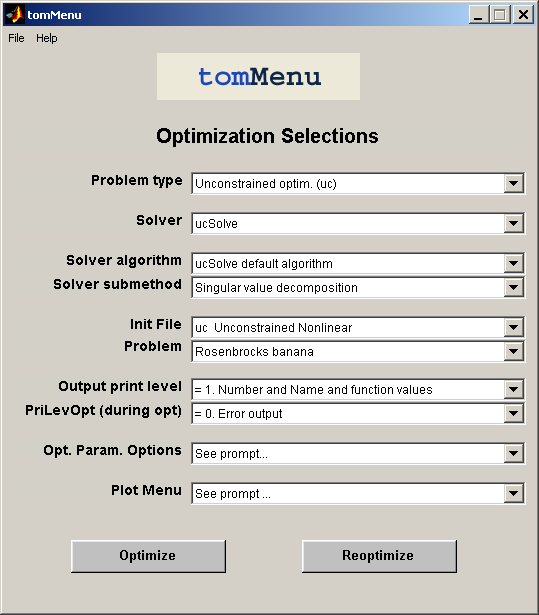
Figure 4: The tomMenu interface.
The Init File pop-down shows the Init File options to the user.
Selecting
lp Linear Programming displays the problems
available.
Note that if the test problems described in this chapter has been
run, there are two more entries in the Init File pop-down menu,
lp Large set of randomized LP problems and
lp
Users Guide LP test problems. If selecting
lp Users Guide
LP test problems the single problem
lpExample will be
selected. If clicking on the button
lp Large set of
randomized LP problems a selection of one of the three different
problems defined is then possible.
After selecting the problem the optimization solver can be
specified. It may also be several algorithms and methods available
for each solver.
The default settings of the optimization parameters are changed by
selecting
Optimization Parameter Options. Pushing the
Optimize button will call the driver routine
tomRun with the solver selected and the result will be
displayed in the Matlab command window.
Instead of using the menu system, the problem could be solved
by a direct call to
tomRun from the Matlab prompt
or as a command in an m-file.
The most straightforward way of doing it (when the problem is defined in
lpnew_prob.m ) is to give the following call from the Matlab prompt:
probNumber = 13; % Assume problem 13 is defined in lpnew_prob
Result = tomRun('lpSimplex','lpnew_prob', probNumber);
Some other possibilities: Assume that a solution of a problem with
the following requirements are wanted:
-
Start in the point (1,1).
- No output printed, neither in the driver routine nor in the solver.
Then the call to
tomRun should be:
 Prob           = probInit('lpnew_prob',13); % Use Init File to define Prob
 PriLev         = 0;
 Prob.x_0       = [1;1];
 Prob.PriLevOpt = 0;
 Result         = tomRun('lp', Prob, PriLev);
To have the result of the optimization displayed call
the routine
PrintResult :
PrintResult(Result);
The following example shows how to call
tomRun
to solve the first problem in
ownlp_prob.m .
Assume the same requirements as the previous problem,
but increase print level to get printing of results
 probFile             = 'ownlp_prob';
 Prob = probInit(probFile,1);
 PriLev               = 2;
 Prob.x_0 = [1;1];
 Prob.optParam.PriLev = 0;
 Result               = tomRun('lp', Prob, PriLev);
5.2 Quadratic Programming Problems
The general formulation in TOMLAB for a quadratic programming problem
is
|
|
|
|
| |
|
| s/t |
| xL |
≤ |
x |
≤ |
xU, |
| bL |
≤ |
A x |
≤ |
bU |
|
|
(14) |
where
c,
x,
xL,
xU Rn,
F Rn × n,
A Rm1 × n, and
bL,
bU Rm1.
Equality constraints are defined by setting
the lower bound equal to the upper bound, i.e.
for constraint
i:
bL(
i) =
bU(
i).
Fixed variables are handled the same way.
To illustrate the solution of QPs consider
the simple quadratic programming test problem
|
|
|
f(x)=4x12+1x1x2+4x22+3x1−4x2 |
| s/t |
x1+x2 ≤ 5 |
| |
x1−x2 = 0 |
| |
x1 ≥ 0 |
| |
x2 ≥ 0, |
|
(15) |
named
QP Example. The following statements define this
problem in Matlab .
File: tomlab/usersguide/qpExample.m
   Name  = 'QP Example';  % File qpExample.m
   F     = [ 8   1        % Matrix F in 1/2 * x' * F * x + c' * x
             1   8 ];
   c     = [ 3  -4 ]';    % Vector c in 1/2 * x' * F * x + c' * x
   A     = [ 1   1        % Constraint matrix
             1  -1 ];
   b_L   = [-inf  0  ]';  % Lower bounds on the linear constraints
   b_U   = [  5   0  ]';  % Upper bounds on the linear constraints
   x_L   = [  0   0  ]';  % Lower bounds on the variables
   x_U   = [ inf inf ]';  % Upper bounds on the variables
   x_0   = [  0   1  ]';  % Starting point
   x_min = [-1 -1 ];      % Plot region lower bound parameters
   x_max = [ 6  6 ];      % Plot region upper bound parameters
5.2.1 A Quick Quadratic Programming solution
The quickest way to solve this problem is to define the following
Matlab statements using the TOMLAB format:
File: tomlab/usersguide/qpTest1.m
qpExample;

Prob = qpAssign(F, c, A, b_L, b_U, x_L, x_U, x_0, 'qpExample');

Result = tomRun('qpSolve', Prob, 1);
The solution of this problem gives the following output to the
screen.
File: tomlab/usersguide/qpTest1.out
===== * * * =================================================================== * * *
TOMLAB SOL+/CGO+/MIN - Three weeks demonstration single user license Valid to 2003-09-20
=====================================================================================
Problem: No Init File    -  1: qpExample        f_k      -0.027777777777777790
                                              f(x_0)      0.000000000000000000

Solver: qpSolve.  EXIT=0.  INFORM=1.
Active set strategy
Optimal point found
First order multipliers >= 0

Iter    4
Starting vector x:
x_0:   0.000000   0.000000
Optimal vector x:
x_k:   0.055556   0.055556
Lagrange multipliers v. Vector length 4:
v_k:  0.000000e+000  0.000000e+000  0.000000e+000  3.500000e+000
Diff x-x0:
      5.555556e-002  5.555556e-002
Gradient g_k:
g_k:  3.500000e+000 -3.500000e+000
Projected gradient gPr: :
gPr:  2.220446e-015 -8.881784e-016
Eigenvalues of Hessian at x_k
eig:   7.000000   9.000000

=== * * * ================================================== * * *
qpAssign is used to define the standard Prob structure, which TOMLAB
always uses to store all information about a problem. The three last
parameters could be left out. The upper bounds will default be Inf,
and the problem name is only used in the printout in
PrintResult to make the output nicer to read. If x_0, the
initial value, is left out, a initial point is found by
qpSolve solving a feasible point (Phase I) linear programming
problem calling the TOMLAB
lpSimplex solver. In fact, the
output shows that the given
x0=(0,−1)
T was rejected because it
was infeasible, and instead a Phase I solution lead to the initial
point
x0=(0,0)
T.
5.2.2 Several Quadratic Programs
If the user wants to solve more than one QP, or maybe the same QP
but under different conditions, then it is possible to define the
problems in the TOMLAB Init File directly. The
qpAssign has additional
functionality and may create an Init File as an option. The file
is then easily added to the GUI data base, and accessible from the
GUI and menu system.
Using the same example (
15) to illustrate this feature gives
File: tomlab/usersguide/qpTest2.m
qpExample;

if exist('qptest.m')   % Remove qptest if it previously exists
   d=which('qptest');
   delete(d);
end

qpAssign(F, c, A, b_L, b_U, x_L, x_U, x_0, 'qpExample', ...
        'qptest',1,[],x_min,x_max);

AddProblemFile('qptest','Users Guide QP test problems','qp');

tomRun('qpSolve','qptest',1);
In this example
more parameters are used in the call to
qpAssign ,
which tells
qpAssign
to define a new TOMLAB Init File called
qptest .
The last two extra parameters
x_min
and
x_max defines initial plotting axis and are efficient when
the user wants to see plots
in the GUI and menu programs. Otherwise these parameters are not needed.
The default is to use the lower and upper bounds on the variables, if
they have finite values.
The
qptest problem file is included as a test file by the call
to
AddProblemFile
and
further set as the default file for QP problems.
Calling
tomRun
to solve the first problem in
qptest
will give exactly the same output as in the first example
in Section
5.2.1.
In the call to
qpAssign the parameter after the file name
qptest , called
nProblem , controls which of two types
of definition files are created (See
help qpAssign
). Setting this parameter as empty or one, as in this case,
defines an open structure in
qptest where the user easily
can insert more test problems. Note the comments in the created
file, which guides the user in how to define a new problem. There
are two places to edit. The name of the new problem must be added
to the
probList string matrix definition on row 17-21, and
then the actual problem definition from row 61 and afterwards. The
new problem definition can be loaded by execution of a script, by
reading from a stored file or the user can explicitly write the
Matlab statements to define the problem in the file
qptest.m . For more information on how to edit a QP Init File,
see the Section
D.2. The other type of QP
definition file created by
qpAssign is discussed in detail
in Section
5.2.3.
When doing this automatic Init File generation
qpAssign stores the problem in a mat-file with a name
combined by three items, the name of the problem file (
qptest ),
the string '_P' and the problem number given as the input parameter
next after the problem file name. In this case
qpAssign defines the file
qptest_P1.mat .
5.2.3 Large Sets of Quadratic Programs
It is easy to create an Init File for a large set
of test problems.
This feature is illustrated
by running a test where the
test problem is disturbed by random noise.
The matrix
F and the vector
c in the objective function are
disturbed,
and the new problems are defined and stored in
the TOMLAB Init File.
To avoid too much output restrict the large number of test
problems to be three.
File: tomlab/usersguide/qpTest3.m
LargeNumber=3;

qpExample;

n=length(c);

if exist('qplarge')   % Remove qplarge if it previously exists
   d=which('qplarge');
   delete(d);
end

for i=1:LargeNumber
    cNew =c + 0.1*(rand(n,1)-0.5);  % Generate random disturbances to vector c
    FNew =F + 0.05*(rand(n,n)-0.5); % Generate random disturbances to matrix F
    FNew =(F + F')/2;               % Make FNew symmetric

    if i==1
       % qpAssign defines qplarge.m for LargeNumber testproblems
       % and stores the first problem in qplarge_P1.mat
       k=[1,LargeNumber];
    else
       k=i; % qpAssign stores the ith problem in the qplarge_Pi.mat problem file
    end

    qpAssign(FNew, cNew, A, b_L, b_U, x_L, x_U, [], Name,'qplarge', k);
end

% Define qplarge as the default file for QP problems in TOMLAB.

AddProblemFile('qplarge','Large set of randomized QP problems','qp');

runtest('qpSolve',0,'qplarge',1:LargeNumber,0,0,1);
Each problem gets a unique name. In the first iteration,
i=1,
qpAssign defines an Init File with three test problems,
and defines the first test problem, stored in
qplarge_P1.mat .
In the other iterations
qpAssign just defines the other mat-files.
All together three mat-files are defined:
qplarge_P1.mat ,
qplarge_P2.mat
and
qplarge_P3.mat .
AddProblemFile adds the new
qplarge problem as
the default QP test problem in TOMLAB .
The
runtest test program utility runs the
selected problems, in this case all three defined.
The second zero argument is used if the actual solver has several
algorithmic options. In this case the zero refers to the default
option, and the only option, in
qpSolve .
The last arguments are used to lower the default output and avoid a
pause statement after each problem is solved.
The results are shown in the following file listing.
File: tomlab/usersguide/qpTest3.out
Solver: qpSolve. Algorithm 0
===== * * * =================================================================== * * *
TOMLAB SOL+/CGO+/MIN - Three weeks demonstration single user license      Valid to 2003-09-20
=====================================================================================
Problem: qplarge -  1: QP Example - 1           f_k      -0.027694057239663620

Solver: qpSolve.  EXIT=0.  INFORM=1.
Active set strategy
Optimal point found
First order multipliers >= 0

FuncEv    4 GradEv    4 ConstrEv    4 Iter    4
CPU time: 0.031000 sec. Elapsed time: 0.031000 sec.
===== * * * =================================================================== * * *
TOMLAB SOL+/CGO+/MIN - Three weeks demonstration single user license      Valid to 2003-09-20
=====================================================================================
Problem: qplarge -  2: QP Example - 2           f_k      -0.021808805588788130

Solver: qpSolve.  EXIT=0.  INFORM=1.
Active set strategy
Optimal point found
First order multipliers >= 0

FuncEv    4 GradEv    4 ConstrEv    4 Iter    4
CPU time: 0.016000 sec. Elapsed time: 0.015000 sec.
===== * * * =================================================================== * * *
TOMLAB SOL+/CGO+/MIN - Three weeks demonstration single user license      Valid to 2003-09-20
=====================================================================================
Problem: qplarge -  3: QP Example - 3           f_k      -0.023503493112249588

Solver: qpSolve.  EXIT=0.  INFORM=1.
Active set strategy
Optimal point found
First order multipliers >= 0

FuncEv    4 GradEv    4 ConstrEv    4 Iter    4
CPU time: 0.016000 sec. Elapsed time: 0.015000 sec.
5.2.4 Another Direct Approach to a QP Solution
The following example shows yet another way to define and solve
the quadratic programming problem (
15) by a direct call
to the routine
qpSolve . The approach is to define a default
Prob structure calling
ProbDef , and then just insert
values into the fields.
 Prob      = ProbDef;
 Prob.QP.F = [ 8   2      % Hessian.
               2   8 ];
 Prob.QP.c = [ 3  -4 ]';  % Constant vector.
 Prob.x_L  = [ 0   0 ]';  % Lower bounds on the variables
 Prob.x_U  = [inf inf]';  % Upper bounds on the variables
 Prob.x_0  = [ 0   1 ]';  % Starting point
 Prob.A    = [ 1   1      % Constraint matrix
               1  -1 ];
 Prob.b_L  = [-inf  0 ]'; % Lower bounds on the constraints
 Prob.b_U  = [  5   0 ]'; % Upper bounds on the constraints
 Result    = tomRun('qpSolve', Prob, 1);
A similar approach is possible when solving all types of problems
in TOMLAB .
5.2.5 More on Solving Quadratic Programs
When the problem is defined in the TOMLAB Init File, it is then possible to run
the graphical user interface
tomGUI , the menu program
tomMenu , or the multi-solver driver routine
tomRun
with the necessary arguments. To call the menu system, type
tomMenu; at the Matlab prompt, choose
Quadratic
Programming The usage is very similar to the solution of Linear
Programs, see the discussion and figures in Section
5.1.4.
5.3 Mixed-Integer Programming Problems
This section describes how to solve mixed-integer programming problems
efficiently using TOMLAB .
To illustrate the solution of MIPs consider
the simple knapsack 0/1 test problem
Weingartner 1, which has 28 binary variables and two knapsacks.
The problem is defined
where
b=(600, 600)
T,
| c = −( |
1898 |
440 |
22507 |
270 |
14148 |
3100 |
4650 |
30800 |
615 |
4975 |
1160 |
4225 |
510 |
11880 |
|
| |
479 |
440 |
490 |
330 |
110 |
560 |
24355 |
2885 |
11748 |
4550 |
750 |
3720 |
1950 |
10500 |
)T |
and the A matrix is


 |
|
| 45 |
0 |
85 |
150 |
65 |
95 |
30 |
0 |
170 |
0 |
40 |
25 |
20 |
0 |
0 |
25 |
0 |
0 |
25 |
0 |
| 165 |
0 |
85 |
0 |
0 |
0 |
0 |
100 |
| 30 |
20 |
125 |
5 |
80 |
25 |
35 |
73 |
12 |
15 |
15 |
40 |
5 |
10 |
10 |
12 |
10 |
9 |
0 |
20 |
| 60 |
40 |
50 |
36 |
49 |
40 |
19 |
150 |
|
|


 |
The following statements define this problem in Matlab
using the TOMLAB format:
File: tomlab/usersguide/mipExample.m
   Name='Weingartner 1 - 2/28 0-1 knapsack';
   % Problem formulated as a minimum problem
   A = [ 45      0     85     150     65     95     30      0    170  0 ...
         40     25     20       0      0     25      0      0     25  0 ...
         165     0     85       0      0      0      0    100  ; ...
         30     20    125       5     80     25     35     73     12  15 ...
         15     40      5      10     10     12     10      9      0  20 ...
         60     40     50      36     49     40     19    150];
   b_U = [600;600];  % 2 knapsack capacities
   c   = [1898  440  22507   270  14148  3100  4650  30800   615  4975 ...
          1160 4225    510 11880    479   440   490    330   110   560 ...
         24355 2885  11748  4550    750  3720  1950  10500]'; % 28 weights

   % Make problem on standard form for mipSolve
   [m,n]   = size(A);
   A       = [A eye(m,m)];
   c       = [-c;zeros(m,1)]; % Change sign to make a minimum problem
   [mm nn] = size(A);
   x_L     = zeros(nn,1);
   x_U     = [ones(n,1);b_U];
   x_0     = [zeros(n,1);b_U];

   fprintf('Knapsack problem. Variables %d. Knapsacks %d\n',n,m);
   fprintf('Making standard form with   %d variables\n',nn);

   % All original variables should be integer, but also slacks in this case
   IntVars = nn;  % Could also be set as: IntVars=1:nn; or IntVars=ones(nn,1);
   x_min   = x_L; x_max  = x_U; f_Low  = -1E7; % f_Low <= f_optimal must hold
   n       = length(c);
   b_L     = b_U;
   f_opt   = -141278;
The quickest way to solve this problem is to define the following
Matlab statements:
File: tomlab/usersguide/mipTest1.m
mipExample;

nProblem  = 7;  % Use the same problem number as in mip_prob.m
fIP       = []; % Do not use any prior knowledge
xIP       = []; % Do not use any prior knowledge
setupFile = []; % Just define the Prob structure, not any permanent setup file
x_opt     = []; % The optimal integer solution is not known
VarWeight = []; % No variable priorities, largest fractional part will be used
KNAPSACK  = 0;  % First run without the knapsack heuristic

Prob = mipAssign(c, A, b_L, b_U, x_L, x_U, x_0, Name, setupFile, nProblem,...
                 IntVars, VarWeight, KNAPSACK, fIP, xIP, ...
                 f_Low, x_min, x_max, f_opt, x_opt);

Prob.Solver.Alg       = 2;    % Depth First, then Breadth (Default Depth First)
Prob.optParam.MaxIter = 5000; % Must increase iterations from default 500
Prob.optParam.IterPrint = 0;
Prob.PriLev = 1;
Result                = tomRun('mipSolve', Prob, 0);

% ------------------------------------------------
% Add priorities on the variables
% ------------------------------------------------
VarWeight = c;
% NOTE. Prob is already defined,  could skip mipAssign, directly set:
% Prob.MIP.VarWeight=c;

Prob = mipAssign(c, A, b_L, b_U, x_L, x_U, x_0, Name, setupFile, nProblem,...
                 IntVars, VarWeight, KNAPSACK, fIP, xIP, ...
                 f_Low, x_min, x_max, f_opt, x_opt);


Prob.Solver.Alg       = 2;             % Depth First, then Breadth search
Prob.optParam.MaxIter = 5000;          % Must increase number of iterations
Prob.optParam.IterPrint = 0;
Prob.PriLev = 1;
Result                = tomRun('mipSolve', Prob, 0);

% ----------------------------------------------
% Use the knapsack heuristic, but not priorities
% ----------------------------------------------
KNAPSACK  = 1; VarWeight = [];
% NOTE. Prob is already defined,  could skip mipAssign, directly set:
% Prob.MIP.KNAPSACK=1;
% Prob.MIP.VarWeight=[];

Prob      = mipAssign(c, A, b_L, b_U, x_L, x_U, x_0, Name, setupFile, ...
                      nProblem, IntVars, VarWeight, KNAPSACK, fIP, xIP, ...
                      f_Low, x_min, x_max, f_opt, x_opt);

Prob.Solver.Alg = 2;              % Depth First, then Breadth search
Prob.optParam.IterPrint = 0;
Prob.PriLev = 1;
Result                = tomRun('mipSolve', Prob, 0);

% --------------------------------------------------
% Now use both the knapsack heuristic and priorities
% --------------------------------------------------
VarWeight = c; KNAPSACK  = 1;
% NOTE. Prob is already defined,  could skip mipAssign, directly set:
% Prob.MIP.KNAPSACK=1;
% Prob.MIP.VarWeight=c;

Prob = mipAssign(c, A, b_L, b_U, x_L, x_U, x_0, Name, setupFile, nProblem,...
                 IntVars, VarWeight, KNAPSACK, fIP, xIP, ...
                 f_Low, x_min, x_max, f_opt, x_opt);

Prob.Solver.Alg = 2;              % Depth First, then Breadth search
Prob.optParam.IterPrint = 0;
Prob.PriLev = 1;
Result                = tomRun('mipSolve', Prob, 0);
To make it easier to see all variable settings, the first lines
define the needed variables. Several of them are just empty
arrays, and could be directly set as empty in the call to
mipAssign .
mipAssign is used to define the standard
Prob structure, which TOMLAB always uses to store all
information about a problem. After mipAssign has defined the
structure
Prob it is then easy to set or change fields in
the structure. The solver
mipSolve is using three different
strategies to search the branch-and-bound tree. The default is the
Depth first strategy, which is also the result if setting
the field
Solver.Alg as zero. Setting the field as one gives
the
Breadth first strategy and setting it as two gives the
Depth first, then breadth search strategy. In the example
our choice is the last strategy. The number of iterations might be
many, thus the maximal number of iterations must be increased, the
field
optParam.MaxIter.
Tests show two ways to improve the convergence of MIP problems.
One is to define a priority order in which the different
non-integer variables are selected as variables to branch on. The
field
MIP.VarWeight is used to set priority numbers for each
variable. Note that the lower the number, the higher the priority.
In our test case the coefficients of the objective function is
used as priority weights. The other way to improve convergence is
to use a heuristic. For binary variables a simple knapsack
heuristic is implemented in
mipSolve . Setting the field
MIP.KNAPSACK as true instructs
mipSolve to use the
heuristic.
Running the four different tests on the knapsack problem
gives the following output to the screen
File: tomlab/usersguide/mipTest1.out
mipTest1
Knapsack problem. Variables 28. Knapsacks 2
Branch and bound. Depth First, then Breadth.

--- Branch & Bound converged! Iterations (nodes visited) =   714 Total LP Iterations =    713

    Optimal Objective function =    -141278.0000000000000000
x: 0  0  1 -0  1  1  1  1  0  1  0  1  1  1
   0  0  0  0  1  0  1  0  1  1  0  1  0  0
B: -1 -1 -1 -1 -1 -1 -1 -1 -1 -1 -1 -1 -1 -1 -1 -1 -1 -1 -1 -1 -1 -1 -1 -1 -1 -1 -1 -1
Branch & bound. Depth First, then Breadth. Priority weights.

--- Branch & Bound converged! Iterations (nodes visited) =   470 Total LP Iterations =    469

    Optimal Objective function =    -141278.0000000000000000
x: 0  0  1 -0  1  1  1  1  0  1  0  1  1  1
   0  0  0  0  1  0  1  0  1  1  0  1  0  0
B: -1 -1 -1 -1 -1 -1 -1 -1 -1 -1 -1 -1 -1 -1 -1 -1 -1 -1 -1 -1 -1 -1 -1 -1 -1 -1 -1 -1
Branch and bound. Depth First, then Breadth. Knapsack Heuristic.
    Found new BEST Knapsack. Nodes left      0. Nodes deleted      0.
    Best IP function value          -139508.0000000000000000
    Found new BEST Knapsack. Nodes left      1. Nodes deleted      0.
    Best IP function value          -140768.0000000000000000
    Found new BEST Knapsack. Nodes left      4. Nodes deleted      0.
    Best IP function value          -141278.0000000000000000

--- Branch & Bound converged! Iterations (nodes visited) =    96 Total LP Iterations =     95

    Optimal Objective function =    -141278.0000000000000000
x: 0  0  1 -0  1  1  1  1  0  1  0  1  1  1
   0  0  0  0  1  0  1  0  1  1  0  1  0  0
B: 1 1 -1 1 -1 -1 -1 -1 1 -1 0 -1 -1 -1 1 1 1 1 -1 1 -1 0 -1 -1 1 -1 -1 1
Branch & bound. Depth First, then Breadth. Knapsack heuristic. Priority weights.
    Found new BEST Knapsack. Nodes left      0. Nodes deleted      0.
    Best IP function value          -139508.0000000000000000
    Found new BEST Knapsack. Nodes left      1. Nodes deleted      0.
    Best IP function value          -140768.0000000000000000
    Found new BEST Knapsack. Nodes left      4. Nodes deleted      0.
    Best IP function value          -141278.0000000000000000

--- Branch & Bound converged! Iterations (nodes visited) =    94 Total LP Iterations =     93

    Optimal Objective function =    -141278.0000000000000000
x: 0  0  1 -0  1  1  1  1  0  1  0  1  1  1
   0  0  0  0  1  0  1  0  1  1  0  1  0  0
B: 1 1 -1 1 -1 -1 -1 -1 1 -1 0 -1 -1 -1 1 1 1 1 -1 1 -1 0 -1 -1 1 -1 -1 1
diary off
Note that there is a large difference in the number of iterations if
the additional heuristic and priorities are used.
Similar results are obtained if running the other two tree
search strategies.
5.3.1 Large Sets of Mixed-Integer Programs
It is easy to setup a problem definition file for a large set
of mixed-integer problems.
The approach is similar to the one for Linear Programs discussed
in Section
5.1.3, the main difference is that
mipAssign
is used instead of
lpAssign .
5.3.2 More on Solving Mixed-Integer Programs
When the problem is defined in the TOMLAB Init File, it is then possible to run
the graphical user interface
tomGUI , the menu program
tomMenu , or the multi-solver driver routine
tomRun
with the necessary arguments. To call the menu system, either type
Result = tomMenu; or just
tomMenu;
at the
Matlab prompt, choose
Mixed-Integer Programming. The usage
is very similar to the solution of Linear Programs, see the
discussion and figures in Section
5.1.4.
Instead of using the menu system solve the problem by a direct call
to
tomRun from the Matlab prompt or as a command in an m-file.
This approach is of interest in an testing environment.
The most straightforward way of doing it (when the problem is defined in
mipnew_prob.m ) is to give the following call from the Matlab prompt:
probNumber = 7;
Result = tomRun('mipSolve', 'mipnew_prob', probNumber);
Assume
the problem should be solved with the following requirements:
-
No printing output neither in the driver routine nor in the solver.
- Use solver mipSolve .
Then the call to
tomRun should be:
 Prob           = probInit('mipnew_prob',7);
 PriLev         = 0;
 Prob.PriLevOpt = 0;
 Result         = tomRun('mipSolve', Prob, PriLev);
To have the result of the optimization displayed call
the routine
PrintResult :
PrintResult(Result);
Assume that
the problem to be solved is defined in another
TOMLAB Init File, say
ownmip_prob.m , which is not the default Init File.
The following example shows how to call
tomRun
to solve the first problem in
ownmip_prob.m .
Assume the same requirements as itemized above.
 probFile       = 'ownmip_prob';
 Prob           = probInit(probFile,1);
 PriLev         = 0;
 Prob.x_0       = [1;1];
 Prob.PriLevOpt = 0;
 Result         = tomRun('mipSolve', Prob, PriLev);
« Previous « Start » Next »
