« Previous « Start » Next »

29  Denbigh’s System of Reactions

Dynamic Optimization of Batch Reactors Using Adaptive Stochastic Algorithms 1997, Eugenio F. Carrasco, Julio R. Banga

Case Study I: Denbigh’s System of Reactions

29.1  Problem description

This optimal control problem is based on the system of chemical reactions initially considered by Denbigh (1958), which was also studied by Aris (1960) and more recently by Luus (1994):

A + B -> X

A + X -> P

X -> Y

X -> Q

where X is an intermediate, Y is the desired product, and P and Q are waste products. This system is described by the following differential equations:

dx1 dt

= −k1*x1−k2*x1

dx2 dt

= k1*x1−k3+k4*x2

dx3 dt

= k3*x2

where x1 = [A][B], x2 = [X] and x3 = [Y]. The initial condition is

x(t0) = [1  0  0]′

The rate constants are given by

ki = ki0*exp(−

Ei R*T

), i=1,2,3,4

where the values of ki0 and Ei are given by Luus (1994).

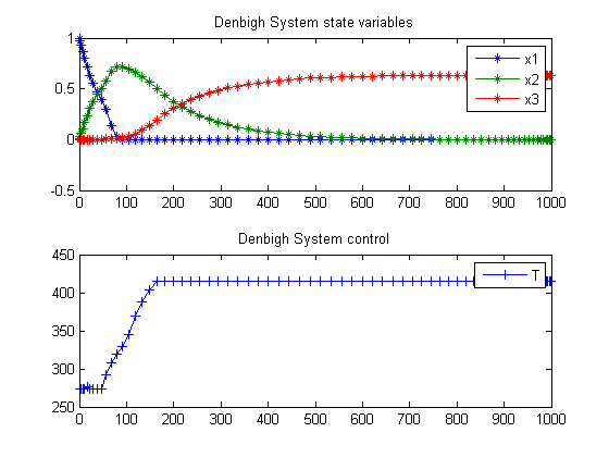
The optimal control problem is to find T(t) (the temperature of the reactor as a function of time) so that the yield of Y is maximized at the end of the given batch time t_f. Therefore, the performance index to be maximized is

J = x3(tf)

where the batch time t_f is specified as 1000 s. The constraints on the control variable (reactor temperature) are

273 <= T <= 415

Reference: [10]

29.2  Problem setup

toms t

29.3  Solve the problem, using a successively larger number collocation points

for n=[25 70]

    p = tomPhase('p', t, 0, 1000, n);
    setPhase(p);
    tomStates x1 x2 x3
    tomControls T

    % Initial guess
    if n==25
        x0 = {icollocate({
            x1 == 1-t/1000;
            x2 == 0.15
            x3 == 0.66*t/1000
            })
            collocate(T==273*(t<100)+415*(t>=100))};
    else
        x0 = {icollocate({
            x1 == x1_init
            x2 == x2_init
            x3 == x3_init
            })
            collocate(T==T_init)};
    end

    % Box constraints
    cbox = {
        0 <= icollocate(x1) <= 1
        0 <= icollocate(x2) <= 1
        0 <= icollocate(x3) <= 1
        273 <= collocate(T) <= 415};

    % Boundary constraints
    cbnd = initial({x1 == 1; x2 == 0
        x3 == 0});

    % Various constants and expressions
    ki0 = [1e3; 1e7; 10; 1e-3];
    Ei  = [3000; 6000; 3000; 0];
    ki4 = ki0(4)*exp(-Ei(4)./T);
    ki3 = ki0(3)*exp(-Ei(3)./T);
    ki2 = ki0(2)*exp(-Ei(2)./T);
    ki1 = ki0(1)*exp(-Ei(1)./T);

    % ODEs and path constraints
    ceq = collocate({
        dot(x1) == -ki1.*x1-ki2.*x1
        dot(x2) == ki1.*x1-(ki3+ki4).*x2
        dot(x3) == ki3.*x2});

    % Objective
    objective = -final(x3);

29.4  Solve the problem

    options = struct;
    options.name = 'Denbigh System';
    solution = ezsolve(objective, {cbox, cbnd, ceq}, x0, options);
    x1_init  = subs(x1,solution);
    x2_init  = subs(x2,solution);
    x3_init  = subs(x3,solution);
    T_init   = subs(T,solution);

Problem type appears to be: lpcon
Starting numeric solver
===== * * * =================================================================== * * *
TOMLAB - Tomlab Optimization Inc. Development license  999001. Valid to 2011-02-05
=====================================================================================
Problem: ---  1: Denbigh System                 f_k      -0.633847592419796270
                                       sum(|constr|)      0.000000569070071108
                              f(x_k) + sum(|constr|)     -0.633847023349725200
                                              f(x_0)     -0.660000000000000140

Solver: snopt.  EXIT=0.  INFORM=1.
SNOPT 7.2-5 NLP code
Optimality conditions satisfied

FuncEv    1 ConstrEv   14 ConJacEv   14 Iter   11 MinorIter 1033
CPU time: 0.140625 sec. Elapsed time: 0.140000 sec.

Problem type appears to be: lpcon
Starting numeric solver
===== * * * =================================================================== * * *
TOMLAB - Tomlab Optimization Inc. Development license  999001. Valid to 2011-02-05
=====================================================================================
Problem: ---  1: Denbigh System                 f_k      -0.633520858635351790
                                       sum(|constr|)      0.000526177451453518
                              f(x_k) + sum(|constr|)     -0.632994681183898230
                                              f(x_0)     -0.633848214286008240

Solver: snopt.  EXIT=0.  INFORM=1.
SNOPT 7.2-5 NLP code
Optimality conditions satisfied

FuncEv    1 ConstrEv   20 ConJacEv   20 Iter   13 MinorIter  233
CPU time: 0.437500 sec. Elapsed time: 0.453000 sec.

end

t  = collocate(subs(t,solution));
x1 = collocate(x1_init);
x2 = collocate(x2_init);
x3 = collocate(x3_init);
T  = collocate(T_init);

29.5  Plot result

subplot(2,1,1)
plot(t,x1,'*-',t,x2,'*-',t,x3,'*-');
legend('x1','x2','x3');
title('Denbigh System state variables');

subplot(2,1,2)
plot(t,T,'+-');
legend('T');
title('Denbigh System control');

« Previous « Start » Next »