« Previous « Start » Next »

59  Linear Pendulum

Viscocity Solutions of Hamilton-Jacobi Equations and Optimal Control Problems. Alberto Bressan, S.I.S.S.A, Trieste, Italy.

A linear pendulum problem controlled by an external force.

59.1  Problem Description

Find u over t in [0; 20 ] to maximize:

J = x1(tf)

subject to:

dx1 dt

= x2

dx2 dt

= u−x1

x(t0) = [0  0]

|u| <= 1

Reference: [8]

59.2  Problem setup

toms t
t_f = 20;
p = tomPhase('p', t, 0, t_f, 60);
setPhase(p);

tomStates x1 x2
tomControls u

% Initial guess
x0 = {icollocate({x1 == 0; x2 == 0})
    collocate(u == 0)};

% Box constraints and bounds
cb = {-1 <= collocate(u) <= 1
    initial(x1 == 0)
    initial(x2 == 0)};

% ODEs and path constraints
ceq = collocate({dot(x1) == x2
    dot(x2) == u-x1});

% Objective
objective = -final(x1);

59.3  Solve the problem

options = struct;
options.name = 'Linear Pendulum';
solution = ezsolve(objective, {cb, ceq}, x0, options);
t  = subs(collocate(t),solution);
x1 = subs(collocate(x1),solution);
x2 = subs(collocate(x2),solution);
u  = subs(collocate(u),solution);

Problem type appears to be: lp
Starting numeric solver
===== * * * =================================================================== * * *
TOMLAB - Tomlab Optimization Inc. Development license  999001. Valid to 2011-02-05
=====================================================================================
Problem: ---  1: Linear Pendulum                f_k     -12.612222977985938000
                                       sum(|constr|)      0.000000000003687556
                              f(x_k) + sum(|constr|)    -12.612222977982251000
                                              f(x_0)      0.000000000000000000

Solver: CPLEX.  EXIT=0.  INFORM=1.
CPLEX Dual Simplex LP solver
Optimal solution found

FuncEv  206 Iter  206
CPU time: 0.031250 sec. Elapsed time: 0.031000 sec.

59.4  Plot result

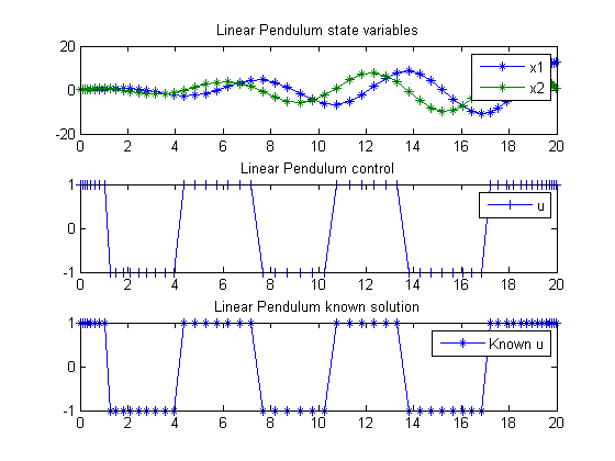
subplot(3,1,1)
plot(t,x1,'*-',t,x2,'*-');
legend('x1','x2');
title('Linear Pendulum state variables');

subplot(3,1,2)
plot(t,u,'+-');
legend('u');
title('Linear Pendulum control');

subplot(3,1,3)
plot(t,sign(sin(t_f-t)),'*-');
legend('Known u');
title('Linear Pendulum known solution');

« Previous « Start » Next »