Singular time-optimal 2 Link robot control
From the paper: L.G. Van Willigenburg, 1991, Computation of time-optimal controls applied to rigid manipulators with friction, Int. J. Contr., Vol. 54, no 5, pp. 1097-1117
Programmers: Gerard Van Willigenburg (Wageningen University) Willem De Koning (retired from Delft University of Technology)
% Array with consecutive number of collocation points
narr = [20 40];

toms t t_f % Free final time

for n=narr
    p = tomPhase('p', t, 0, t_f, n);
    setPhase(p)

    tomStates x1 x2 x3 x4
    tomControls u1 u2

    % Initial & terminal states
    xi = [0;   0; 0; 0];
    xf = [1.5; 0; 0; 0];

    % Initial guess
    if n==narr(1)
        x0 = {t_f==1; icollocate({x1 == xf(1); x2 == xf(2)
            x3 == xf(3); x4 == xf(4)})
            collocate({u1 == 0; u2 == 0})};
    else
        x0 = {t_f==tfopt; icollocate({x1 == xopt1; x2 == xopt2
            x3 == xopt3; x4 == xopt4})
            collocate({u1 == uopt1; u2 == uopt2})};
    end

    % Box constraints
    cbox = {0.75 <= t_f <= 1.5; -25 <= collocate(u1) <= 25
        -9 <= collocate(u2) <= 9};

    % Boundary constraints
    cbnd = {initial({x1 == xi(1); x2 == xi(2)
        x3 == xi(3); x4 == xi(4)})
        final({x1 == xf(1); x2 == xf(2)
        x3 == xf(3); x4 == xf(4)})};

    % ODEs and path constraints
    % Robot parameters
    mm11 = 5.775; mm12 = 0.815; mm22 = 0.815;
    hm11 = 1.35;  m1   = 30.0;  m2   = 15;

    % Variables for dynamics
    c1  = cos(x1);        c2  = cos(x2);
    s2  = sin(x2);        c12 = cos(x1+x2);
    ms1 = mm11+2*hm11*c2; ms2 = mm12+hm11*c2;

    mdet  = ms1.*mm22-ms2.*ms2;
    ms11 = mm22./mdet; ms12=-ms2./mdet; ms22=ms1./mdet;

    qg1 = -hm11*s2.*(x4.*x4+2*x3.*x4);
    qg2 = hm11*s2.*x3.*x3;

    dx1 = x3; dx2=x4;
    dx3 = ms11.*(u1-qg1)+ms12.*(u2-qg2);
    dx4 = ms12.*(u1-qg1)+ms22.*(u2-qg2);

    ceq = collocate({
        dot(x1) == dx1
        dot(x2) == dx2
        dot(x3) == dx3
        dot(x4) == dx4});

    % Objective
    objective = t_f;
    options = struct;
    options.name = '2-Link-Robot';
    solution = ezsolve(objective, {cbox, cbnd, ceq}, x0, options);

    tfopt = subs(t_f,solution);
    xopt1 = subs(x1,solution);
    xopt2 = subs(x2,solution);
    xopt3 = subs(x3,solution);
    xopt4 = subs(x4,solution);
    uopt1 = subs(u1,solution);
    uopt2 = subs(u2,solution);
Problem type appears to be: lpcon
Starting numeric solver
===== * * * =================================================================== * * *
TOMLAB - Tomlab Optimization Inc. Development license  999001. Valid to 2011-02-05
=====================================================================================
Problem: ---  1: 2-Link-Robot                   f_k       1.225664453973471300
                                       sum(|constr|)      0.000003477368351302
                              f(x_k) + sum(|constr|)      1.225667931341822600
                                              f(x_0)      1.000000000000000000

Solver: snopt.  EXIT=0.  INFORM=1.
SNOPT 7.2-5 NLP code
Optimality conditions satisfied

FuncEv    1 ConstrEv 2552 ConJacEv 2552 Iter  568 MinorIter 4959
CPU time: 7.765625 sec. Elapsed time: 7.953000 sec.
Problem type appears to be: lpcon
Starting numeric solver
===== * * * =================================================================== * * *
TOMLAB - Tomlab Optimization Inc. Development license  999001. Valid to 2011-02-05
=====================================================================================
Problem: ---  1: 2-Link-Robot                   f_k       1.223303478413072100
                                       sum(|constr|)      0.000000031552847509
                              f(x_k) + sum(|constr|)      1.223303509965919500
                                              f(x_0)      1.225664453973471300

Solver: snopt.  EXIT=0.  INFORM=1.
SNOPT 7.2-5 NLP code
Optimality conditions satisfied

FuncEv    1 ConstrEv   44 ConJacEv   44 Iter   16 MinorIter  358
CPU time: 0.406250 sec. Elapsed time: 0.406000 sec.
end
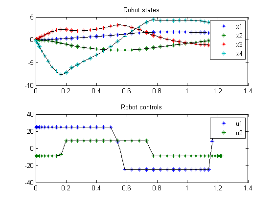
figure(1)
subplot(2,1,1);
ezplot([x1; x2; x3; x4]); legend('x1','x2','x3','x4');
title('Robot states');
subplot(2,1,2);
ezplot([u1; u2]); legend('u1','u2');
title('Robot controls');