« Previous « Start » Next »

96  Second Order System

Users Guide for dyn.Opt, Example 1

Optimal control of a second order system

End time says 1 in problem text.

96.1  Problem Formulation

Find u over t in [0; 2 ] to minimize

J =

∫

2 0

u2/2 dt

subject to:

dx1 dt

= x2

dx2 dt

= u

x1(0) = 1

x1(2) = 0

x2(0) = 1

x2(2) = 0

−100 <= u <= 100

Reference: [16]

96.2  Problem setup

toms t
p = tomPhase('p', t, 0, 2, 30);
setPhase(p);

tomStates x1 x2
tomControls u

% Initial guess
x0 = {icollocate({x1 == 1-t/2; x2 == -1+t/2})
    collocate(u == -3.5+6*t/2)};

% Box constraints
cbox = {-100 <= icollocate(x1) <= 100
    -100 <= icollocate(x2) <= 100
    -100 <= collocate(u)   <= 100};

% Boundary constraints
cbnd = {initial({x1 == 1; x2 == 1})
    final({x1 == 0; x2 == 0})};

% ODEs and path constraints
ceq = collocate({dot(x1) == x2; dot(x2) == u});

% Objective
objective = integrate(u.^2/2);

96.3  Solve the problem

options = struct;
options.name = 'Second Order System';
solution = ezsolve(objective, {cbox, cbnd, ceq}, x0, options);
t  = subs(collocate(t),solution);
x1 = subs(collocate(x1),solution);
x2 = subs(collocate(x2),solution);
u  = subs(collocate(u),solution);

Problem type appears to be: qp
Starting numeric solver
===== * * * =================================================================== * * *
TOMLAB - Tomlab Optimization Inc. Development license  999001. Valid to 2011-02-05
=====================================================================================
Problem:  1: Second Order System                f_k       3.249999999996386900
                                       sum(|constr|)      0.000000000432709878
                              f(x_k) + sum(|constr|)      3.250000000429096800
                                              f(x_0)      0.000000000000000000

Solver: CPLEX.  EXIT=0.  INFORM=1.
CPLEX Barrier QP solver
Optimal solution found

FuncEv    6 GradEv    6 ConstrEv    6 Iter    6
CPU time: 0.015625 sec. Elapsed time: 0.016000 sec.

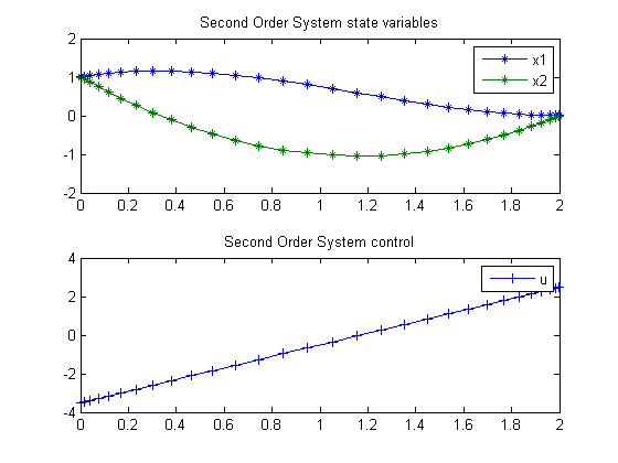
96.4  Plot result

subplot(2,1,1)
plot(t,x1,'*-',t,x2,'*-');
legend('x1','x2');
title('Second Order System state variables');

subplot(2,1,2)
plot(t,u,'+-');
legend('u');
title('Second Order System control');

« Previous « Start » Next »