« Previous « Start » Next »

71  Nishida problem

Second-order sensitivities of general dynamic systems with application to optimal control problems. 1999, Vassilios S. Vassiliadis, Eva Balsa Canto, Julio R. Banga

Case Study 6.3: Nishida problem

71.1  Problem description

This case study was presented by Nishida et al. (1976) and it is posed as follows:

Minimize:

J = x1(tf)2+x2(tf)2+x3(tf)2+x4(tf)2

subject to:

dx1 dt

= −0.5*x1+5*x2

dx2 dt

= −5*x1−0.5*x2+u

dx3 dt

= −0.6*x3+10*x4

dx4 dt

= −10*x3−0.6*x4+u

−1.0 <= u <= 1.0

with the initial conditions: x(i) = 10, i=1,..,4 and with t_f = 4.2.

Reference: [31]

71.2  Problem setup

toms t
p = tomPhase('p', t, 0, 4.2, 60);
setPhase(p);

tomStates x1 x2 x3 x4
tomControls u

% Initial guess
x0 = {icollocate({
    x1 == 10-10*t/4.2; x2 == 10-10*t/4.2
    x3 == 10-10*t/4.2; x4 == 10-10*t/4.2})
    collocate(u == 0)};

% Box constraints
cbox = {icollocate({
    -15 <= x1 <= 15; -15 <= x2 <= 15
    -15 <= x3 <= 15; -15 <= x4 <= 15})
    -1  <= collocate(u) <= 1};

% Boundary constraints
cbnd = initial({x1 == 10; x2 == 10
    x3 == 10; x4 == 10});

% ODEs and path constraints
ceq = collocate({
    dot(x1) == -0.5*x1+5*x2
    dot(x2) == -5*x1-0.5*x2+u
    dot(x3) == -0.6*x3+10*x4
    dot(x4) == -10*x3-0.6*x4+u});

% Objective
objective = final(x1)^2+final(x2)^2+final(x3)^2+final(x4)^2;

71.3  Solve the problem

options = struct;
options.name = 'Nishida Problem';
solution = ezsolve(objective, {cbox, cbnd, ceq}, x0, options);
t  = subs(collocate(t),solution);
x1 = subs(collocate(x1),solution);
x2 = subs(collocate(x2),solution);
x3 = subs(collocate(x3),solution);
x4 = subs(collocate(x4),solution);
u  = subs(collocate(u),solution);

Problem type appears to be: qp
Starting numeric solver
===== * * * =================================================================== * * *
TOMLAB - Tomlab Optimization Inc. Development license  999001. Valid to 2011-02-05
=====================================================================================
Problem:  1: Nishida Problem                    f_k       1.004684962685394000
                                       sum(|constr|)      0.000018521427591828
                              f(x_k) + sum(|constr|)      1.004703484112985800
                                              f(x_0)      0.000000000000000000

Solver: CPLEX.  EXIT=0.  INFORM=1.
CPLEX Barrier QP solver
Optimal solution found

FuncEv   15 GradEv   15 ConstrEv   15 Iter   15
CPU time: 0.140625 sec. Elapsed time: 0.125000 sec.

71.4  Plot result

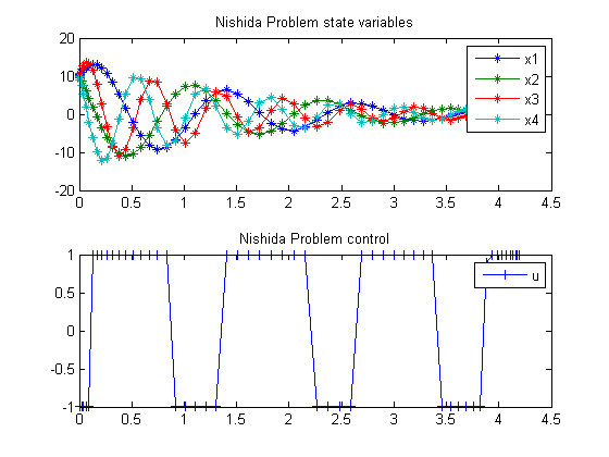
subplot(2,1,1)
plot(t,x1,'*-',t,x2,'*-',t,x3,'*-',t,x4,'*-');
legend('x1','x2','x3','x4');
title('Nishida Problem state variables');

subplot(2,1,2)
plot(t,u,'+-');
legend('u');
title('Nishida Problem control');

« Previous « Start » Next »