Green House Control Example

46 Greenhouse Climate Control

Greenhouse Optimal Climate Control, a problem with external inputs

46.1 Problem description

Taken from the book: Optimal Control of Greenhouse Cultivation G. van Straten, R.J.C. van Ooteghem, L.G. van Willigenburg, E. van Henten

ISBN: 9781420059618 CRC Pr I Llc Books

Programmers: Gerard Van Willigenburg (Wageningen University)

46.2 Problem setup

% Define tomSym variable t (time) and t_f (fixed final time)
toms t; t_f = 48;

% Define and set time axis
p = tomPhase('p', t, 0, t_f, 50);
setPhase(p);

% Define the state and control variables
tomStates x1 x2 x3
tomControls u
x = [x1; x2; x3];

% Initial state
xi = [0; 10; 0];

% Initial guess
x0 = {icollocate(x == xi); collocate(u == 0)};

% Boundary conditions
cbnd = initial(x == xi);

% Equality constraints: state-space diffenrential equations
pW = 3e-6/40; pT = 1; pH = 0.1;
pHc = 7.5e-2/220; pWc = 3e4/220;

% External inputs: [time, sunlight, outside temperature]
te  = (-1:0.2:49)';
tue = [te 800*sin(4*pi*te/t_f-0.65*pi) 15+10*sin(4*pi*te/t_f-0.65*pi)];

% Extract external inputs from table tue through interpolation
ue1 = interp1(tue(:,1),tue(:,2),t);
ue2 = interp1(tue(:,1),tue(:,3),t);

%Differential equations
ceq = collocate({
    dot(x1) == pW*ue1*x2
    dot(x2) == pT*(ue2-x2)+pH*u;
    dot(x3) == pHc*u});

% Control bounds
cbox = {0 <= collocate(u) <= 10};

% Cost function to be minimized
objective = final(x3-pWc*x1);

46.3 Solve the problem

options = struct;
options.name = 'Greenhouse Problem';
solution = ezsolve(objective, {cbox, cbnd, ceq}, x0, options);

% Obtain final solution t,x1,...,u,..
% that overwrite the associated tomSym variables
t  = subs(collocate(t),solution);
x1 = subs(collocate(x1),solution);
x2 = subs(collocate(x2),solution);
x3 = subs(collocate(x3),solution);
u = subs(collocate(u),solution);

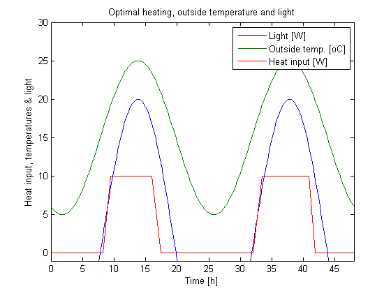
%Plot external inputs and control
figure(1);
plot(tue(:,1),tue(:,2)/40,tue(:,1),tue(:,3),t,u); axis([0 t_f -1 30]);
xlabel('Time [h]');
ylabel('Heat input, temperatures & light');
legend('Light [W]','Outside temp. [oC]','Heat input [W]');
title('Optimal heating, outside temperature and light');

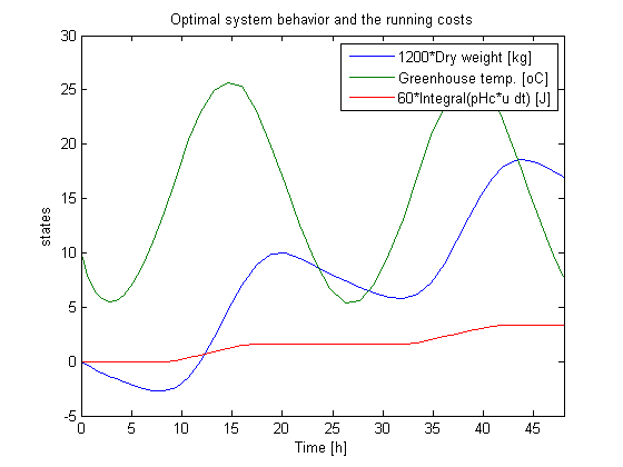
% Plot the optimal state
figure(2)
sf1=1200; sf3=60;
plot(t,[sf1*x1 x2 sf3*x3]); axis([0 t_f -5 30]);
xlabel('Time [h]'); ylabel('states');
legend('1200*Dry weight [kg]','Greenhouse temp. [oC]','60*Integral(pHc*u dt) [J]');
title('Optimal system behavior and the running costs');

Problem type appears to be: lp
Starting numeric solver
===== * * * =================================================================== * * *
TOMLAB - Tomlab Optimization Inc. Development license  999001. Valid to 2011-02-05
=====================================================================================
Problem: ---  1: Greenhouse Problem             f_k      -1.870359095786537500
                                       sum(|constr|)      0.000000000000137357
                              f(x_k) + sum(|constr|)     -1.870359095786400000
                                              f(x_0)      0.000000000000000000

Solver: CPLEX.  EXIT=0.  INFORM=1.
CPLEX Dual Simplex LP solver
Optimal solution found

FuncEv  187 Iter  187
CPU time: 0.031250 sec. Elapsed time: 0.031000 sec.

« Previous « Start » Next »