« Previous « Start » Next »
92 Rigid Body Rotation
On smooth optimal control determination, Ilya Ioslovich and Per-Olof Gutman, Technion, Israel Institute of Technology.
Example 1: Rigid body rotation
92.1 Problem Description
Find u over t in [0; 1 ] to minimize:
subject to:
Reference: [18]
92.2 Problem setup
toms t
p = tomPhase('p', t, 0, 1, 20);
setPhase(p);

tomStates x y u1 u2

% Boundary constraints
cbnd = {initial({x == 0.9; y == 0.75})
    final({x == 0; y == 0})};

% ODEs and path constraints
a = 2;
ceq = collocate({dot(x)  == a*y+u1; dot(y)  == -a*x+u2
    dot(u1) == a*u2; dot(u2) == -a*u1});

% Objective
objective = 0.25*integrate((u1.^2+u2.^2).^2);
92.3 Solve the problem
options = struct;
options.name = 'Rigid Body Rotation';
solution = ezsolve(objective, {cbnd, ceq}, [], options);
t  = subs(collocate(t),solution);
x = subs(collocate(x),solution);
y = subs(collocate(y),solution);
u1 = subs(collocate(u1),solution);
u2 = subs(collocate(u2),solution);
Problem type appears to be: con
Starting numeric solver
===== * * * =================================================================== * * *
TOMLAB - Tomlab Optimization Inc. Development license  999001. Valid to 2011-02-05
=====================================================================================
Problem: ---  1: Rigid Body Rotation            f_k       0.470939062500256130
                                       sum(|constr|)      0.000000000003070916
                              f(x_k) + sum(|constr|)      0.470939062503327070
                                              f(x_0)      0.000000000000000000

Solver: snopt.  EXIT=0.  INFORM=1.
SNOPT 7.2-5 NLP code
Optimality conditions satisfied

FuncEv    3 GradEv    1 MinorIter   39
CPU time: 0.031250 sec. Elapsed time: 0.032000 sec.
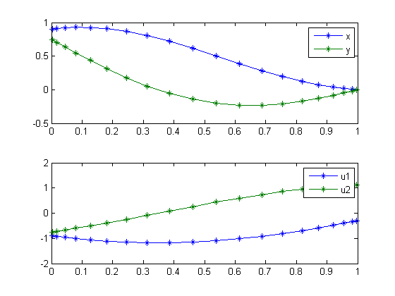
92.4 Plot result
figure(1);
subplot(2,1,1);
plot(t,x,'*-',t,y,'*-');
legend('x','y');

subplot(2,1,2);
plot(t,u1,'*-',t,u2,'*-');
legend('u1','u2');
« Previous « Start » Next »
