a Dynamic Optimization Approach 2009, Diego A. Oyarzuna, Brian P. Ingalls, Richard H. Middleton, Dimitrios Kalamatianosa
The problem is described in the paper referenced above.
N = [30 128]; % Number of collocation points
toms t t_f
warning('off', 'tomSym:x0OutOfBounds');

for n = N
    p = tomPhase('p', t, 0, t_f, n);
    setPhase(p);
    tomStates s1 s2 s3 e0 e1 e2 e3
    tomControls u0 u1 u2 u3

    % Initial guess
    if n == N(1)
        x0 = {t_f == 2
            icollocate({
            [s1;s2;s3] == 0
            e0 == t/t_f
            e1 == (t-0.2)/t_f
            e2 == (t-1)/t_f
            e3 == (t-1.2)/t_f
            })
            collocate({u0 == 1
            [u1;u2;u3] == 0})};
    else
        x0 = {t_f == tf_init
            icollocate({
            s1 == s1_init; s2 == s2_init; s3 == s3_init
            e0 == e0_init; e1 == e1_init; e2 == e2_init
            e3 == e3_init})
            collocate({u0 == u0_init
            u1 == u1_init; u2 == u2_init; u3 == u3_init})};
    end
    % Box constraints
    cbox = {0.1 <= t_f <= tfmax
        0  <= icollocate([s1;s2;s3]) <= 100
        0  <= icollocate([e0;e1;e2;e3]) <= 1
        0  <= collocate([u0;u1;u2;u3])  <= Umax};

    % Boundary constraints
    cbnd = {initial({[s1;s2;s3] == 0; [e0;e1;e2;e3] == 0})
        final({s1 == s1f; s2 == s2f; s3 == s3f;
        e0 == e0f; e1 == e1f; e2 == e2f; e3 == e3f})};

    % Michaelis-Mentes ODEs and path constraints
    ceq = collocate({
        dot(s1) == kcat0*s0*e0/(Km + s0) - kcat1*s1*e1/(Km+s1)
        dot(s2) == kcat1*s1*e1/(Km+s1) - kcat2*s2*e2/(Km+s2)
        dot(s3) == kcat2*s2*e2/(Km+s2) - kcat3*s3*e3/(Km+s3)
        dot(e0) == u0 - lam*e0
        dot(e1) == u1 - lam*e1
        dot(e2) == u2 - lam*e2
        dot(e3) == u3 - lam*e3});

    % Objective
    objective = integrate(1 + e0 + e1 + e2 + e3);
    options = struct;
    options.name = 'Metabolic Pathways, Unbranched n=4';
    solution = ezsolve(objective, {cbox, cbnd, ceq}, x0, options);

    % Collect solution as initial guess
    s1_init = subs(s1,solution);
    s2_init = subs(s2,solution);
    s3_init = subs(s3,solution);
    e0_init = subs(e0,solution);
    e1_init = subs(e1,solution);
    e2_init = subs(e2,solution);
    e3_init = subs(e3,solution);
    tf_init = subs(t_f,solution);
    u0_init = subs(u0,solution);
    u1_init = subs(u1,solution);
    u2_init = subs(u2,solution);
    u3_init = subs(u3,solution);
Problem type appears to be: qpcon
Starting numeric solver
===== * * * =================================================================== * * *
TOMLAB - Tomlab Optimization Inc. Development license  999001. Valid to 2011-02-05
=====================================================================================
Problem: ---  1: Metabolic Pathways, Unbranched n=4  f_k       6.092698010914444900
                                            sum(|constr|)      0.000001117096701837
                                   f(x_k) + sum(|constr|)      6.092699128011147100
                                                   f(x_0)      4.220507512582271300

Solver: snopt.  EXIT=0.  INFORM=1.
SNOPT 7.2-5 NLP code
Optimality conditions satisfied

FuncEv    1 ConstrEv   34 ConJacEv   34 Iter   22 MinorIter 1806
CPU time: 0.734375 sec. Elapsed time: 0.750000 sec.
Problem type appears to be: qpcon
Starting numeric solver
===== * * * =================================================================== * * *
TOMLAB - Tomlab Optimization Inc. Development license  999001. Valid to 2011-02-05
=====================================================================================
Problem: ---  1: Metabolic Pathways, Unbranched n=4  f_k       6.085709091573209100
                                            sum(|constr|)      0.000005873260299532
                                   f(x_k) + sum(|constr|)      6.085714964833508500
                                                   f(x_0)      6.092720075212315400

Solver: snopt.  EXIT=0.  INFORM=1.
SNOPT 7.2-5 NLP code
Optimality conditions satisfied

FuncEv    1 ConstrEv    7 ConJacEv    7 Iter    5 MinorIter 2096
CPU time: 9.343750 sec. Elapsed time: 9.672000 sec.
end

% Collect data
t  = subs(collocate(t),solution);
s1 = subs(collocate(s1),solution);
s2 = subs(collocate(s2),solution);
s3 = subs(collocate(s3),solution);
e0 = subs(collocate(e0),solution);
e1 = subs(collocate(e1),solution);
e2 = subs(collocate(e2),solution);
e3 = subs(collocate(e3),solution);
u0  = subs(collocate(u0),solution);
u1  = subs(collocate(u1),solution);
u2  = subs(collocate(u2),solution);
u3  = subs(collocate(u3),solution);
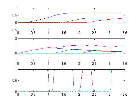
s = [s1 s2 s3];
e = [e0 e1 e2 e3];
r = [u0 u1 u2 u3];
subplot(3,1,1);
plot(t,[s1 s2 s3]);
subplot(3,1,2);
plot(t,[e0 e1 e2 e3 e0+e1+e2+e3]);
subplot(3,1,3);
plot(t,[u0 u1 u2 u3]);