« Previous « Start » Next »
62 Marine Population Dynamics
Benchmarking Optimization Software with COPS Elizabeth D. Dolan and Jorge J. More ARGONNE NATIONAL LABORATORY
62.1 Problem Formulation
Find m and g over t in [0; 10] to minimize
subject to:
Where the data is given in the code.
Reference: [14]
62.2 Problem setup
t = tom('t');
m = tom('m',8,1);
g = tom('g',7,1);

% Various constants and expressions
ymeas = [...
    20000 17000 10000 15000 12000 9000 7000 3000
    12445 15411 13040 13338 13484 8426 6615 4022
     7705 13074 14623 11976 12453 9272 6891 5020
     4664  8579 12434 12603 11738 9710 6821 5722
     2977  7053 11219 11340 13665 8534 6242 5695
     1769  5054 10065 11232 12112 9600 6647 7034
      943  3907  9473 10334 11115 8826 6842 7348
      581  2624  7421 10297 12427 8747 7199 7684
      355  1744  5369  7748 10057 8698 6542 7410
      223  1272  4713  6869  9564 8766 6810 6961
      137   821  3451  6050  8671 8291 6827 7525
       87   577  2649  5454  8430 7411 6423 8388
       49   337  2058  4115  7435 7627 6268 7189
       32   228  1440  3790  6474 6658 5859 7467
       17   168  1178  3087  6524 5880 5562 7144
       11    99   919  2596  5360 5762 4480 7256
        7    65   647  1873  4556 5058 4944 7538
        4    44   509  1571  4009 4527 4233 6649
        2    27   345  1227  3677 4229 3805 6378
        1    20   231   934  3197 3695 3159 6454
        1    12   198   707  2562 3163 3232 5566];

tmeas = 0:0.5:10;

% Box constraints
cbox = {
    0 <= m
    0 <= g
    };

p = tomPhase('p', t, tmeas(1), tmeas(end), 2*length(tmeas), [], 'gauss');
setPhase(p);
y = tomState('y',8,1);

% Initial guess - linear interpolation between the data points
x0 = {m==0; g==0;
    icollocate(y == interp1(tmeas,ymeas,t)')};

yerr = sum(sum((atPoints(tmeas,y) - ymeas).^2));

% ODE
ceq = collocate( dot(y) == [0; g].*[0; y(1:7)] - (m+[g;0]).*y );
62.3 Solve the problem
options = struct;
options.name = 'Marine Population Dynamics';
solution = ezsolve(1e-5*yerr, {cbox, ceq}, x0, options);

% Optimal y, m and g - use as starting guess
yopt = subs(y, solution);
mopt = subs(m, solution);
gopt = subs(g, solution);
Problem type appears to be: qpcon
Starting numeric solver
===== * * * =================================================================== * * *
TOMLAB - Tomlab Optimization Inc. Development license  999001. Valid to 2011-02-05
=====================================================================================
Problem: ---  1: Marine Population Dynamics     f_k     197.465297161281340000
                                       sum(|constr|)      0.000000124069941210
                              f(x_k) + sum(|constr|)    197.465297285351280000
                                              f(x_0) -86874.198350960098000000

Solver: snopt.  EXIT=0.  INFORM=1.
SNOPT 7.2-5 NLP code
Optimality conditions satisfied

FuncEv    1 ConstrEv   15 ConJacEv   15 Iter   14 MinorIter  432
CPU time: 0.718750 sec. Elapsed time: 0.407000 sec.
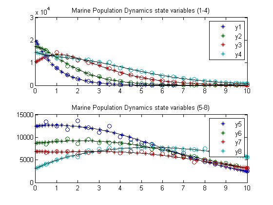
62.4 Plot result
subplot(2,1,1)
ezplot(y(1:4));
hold on
plot(tmeas,ymeas(:,1:4),'o');
hold off
legend('y1','y2','y3','y4');
title('Marine Population Dynamics state variables (1-4)');

subplot(2,1,2)
ezplot(y(5:8));
legend('y5','y6','y7','y8');
hold on
plot(tmeas,ymeas(:,5:8),'o');
hold off
title('Marine Population Dynamics state variables (5-8)');
« Previous « Start » Next »
