« Previous « Start » Next »

51  Hyper Sensitive Optimal Control

Eigenvector approximate dichotomic basis method for solving hyper-sensitive optimal control problems 2000, Anil V. Rao and Kenneth D. Mease

3.1. Motivating example, a hyper-sensitive HBVP

51.1  Problem Formulation

Find u(t) over t in [0; t_f ] to minimize

J =

∫

tf 0

(x2 + u2) dt

subject to:

dx dt

= −x3+u

x0 = 1

xtf = 1.5

tf = 10

Reference: [27]

51.2  Problem setup

toms t
p = tomPhase('p', t, 0, 10, 50);
setPhase(p);

tomStates x
tomControls u

% Initial guess
x0 = {icollocate(x == 0)
    collocate(u == 0)};

% bounds and ODEs
bceq = {collocate(dot(x) == -x.^3+u)
    initial(x) == 1; final(x) == 1.5};

% Objective
objective = integrate(x.^2+u.^2);

51.3  Solve the problem

options = struct;
options.name = 'Hyper Sensitive';
solution = ezsolve(objective, bceq, x0, options);
t = subs(collocate(t),solution);
x = subs(collocate(x),solution);
u = subs(collocate(u),solution);

Problem type appears to be: qpcon
Starting numeric solver
===== * * * =================================================================== * * *
TOMLAB - Tomlab Optimization Inc. Development license  999001. Valid to 2011-02-05
=====================================================================================
Problem: ---  1: Hyper Sensitive                f_k       6.723925391388356800
                                       sum(|constr|)      0.000000002440650080
                              f(x_k) + sum(|constr|)      6.723925393829007100
                                              f(x_0)      0.000000000000000000

Solver: snopt.  EXIT=0.  INFORM=1.
SNOPT 7.2-5 NLP code
Optimality conditions satisfied

FuncEv    1 ConstrEv   26 ConJacEv   26 Iter   21 MinorIter   70
CPU time: 0.093750 sec. Elapsed time: 0.093000 sec.

51.4  Plot result

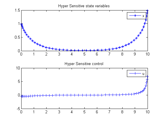
subplot(2,1,1)
plot(t,x,'*-');
legend('x');
title('Hyper Sensitive state variables');

subplot(2,1,2)
plot(t,u,'+-');
legend('u');
title('Hyper Sensitive control');

« Previous « Start » Next »