« Previous « Start » Next »

84  Path Tracking Robot (Two-Phase)

User’s Guide for DIRCOL

2.7 Optimal path tracking for a simple robot. A robot with two rotational joints and simplified equations of motion has to move along a prescribed path with constant velocity.

84.1  Problem Formulation

Find u over t in [0; 2 ] to minimize

J =

∫

2 0

(

2 ∑ i=1

(wi*(qi(t) − qi,ref)2) +

2 ∑ i=1

(w2+i*(

dq dt

i(t) −

dq dt

i,ref)2) dt

subject to:

d2q1 dt2

= u1

d2q2 dt2

= u2

A transformation gives:

dx1 dt

= x3

dx2 dt

= x4

dx3 dt

= u1

dx4 dt

= u2

x1:4(0) = [0  0  0.5  0]

x1:4(2) = [0.5  0.5  0  0.5]

w1:4 = [100  100  500  500]

x11,ref =

t 2

(0<t<1),

1 2

(1<t<2)

x21,ref = 0  (0<t<1),

t−1 2

(1<t<2)

x31,ref =

1 2

(0<t<1),  0  (1<t<2)

x41,ref = 0  (0<t<1),

1 2

(1<t<2)

|u| < 10

Reference: [33]

84.2  Problem setup

t_F = 2;
toms t1
p1 = tomPhase('p1', t1, 0, t_F/2, 25);
toms t2
p2 = tomPhase('p2', t2, t_F/2, t_F/2, 25);
setPhase(p1);

tomStates x1p1 x2p1 x3p1 x4p1
tomControls u1p1 u2p1

% Box constraints
cbox1 = {-10 <= collocate(u1p1) <= 10
    -10 <= collocate(u2p1) <= 10};

% Boundary constraints
w1 = 100; w2 = 100;
w3 = 500; w4 = 500;
err1p1 = w1*(x1p1-t1/2).^2;
err2p1 = w2*(x2p1).^2;
err3p1 = w3*(x3p1-1/2).^2;
err4p1 = w4*(x4p1).^2;

cbnd1 = initial({x1p1 == 0; x2p1 == 0
    x3p1 == 0.5; x4p1 == 0});

% ODEs and path constraints
ceq1 = collocate({dot(x1p1) == x3p1
    dot(x2p1) == x4p1; dot(x3p1) == u1p1
    dot(x4p1) == u2p1});

% Objective
objective1 = integrate(err1p1+err2p1+err3p1+err4p1);

% Phase 2
setPhase(p2);
tomStates x1p2 x2p2 x3p2 x4p2
tomControls u1p2 u2p2

% Box constraints
cbox2 = {-10 <= collocate(u1p2) <= 10
    -10 <= collocate(u2p2) <= 10};

% Boundary constraints
err1p2 = w1*(x1p2-1/2).^2;
err2p2 = w2*(x2p2-(t2-1)/2).^2;
err3p2 = w3*(x3p2).^2;
err4p2 = w4*(x4p2-1/2).^2;

cbnd2 = final({x1p2 == 0.5
    x2p2 == 0.5
    x3p2 == 0
    x4p2 == 0.5});

% ODEs and path constraints
ceq2 = collocate({
    dot(x1p2) == x3p2
    dot(x2p2) == x4p2
    dot(x3p2) == u1p2
    dot(x4p2) == u2p2});

% Objective
objective2 = integrate(err1p2+err2p2+err3p2+err4p2);

% Objective
objective = objective1 + objective2;

% Link phase
link = {final(p1,x1p1) == initial(p2,x1p2)
    final(p1,x2p1) == initial(p2,x2p2)
    final(p1,x3p1) == initial(p2,x3p2)
    final(p1,x4p1) == initial(p2,x4p2)};

84.3  Solve the problem

options = struct;
options.name = 'Path Tracking Robot (Two-Phase)';
options.solver = 'sqopt7';
constr = {cbox1, cbnd1, ceq1, cbox2, cbnd2, ceq2, link};
solution = ezsolve(objective, constr, [], options);
t = subs(collocate(p1,t1),solution);
t = [t;subs(collocate(p2,t2),solution)];
x1 = subs(collocate(p1,x1p1),solution);
x1 = [x1;subs(collocate(p2,x1p2),solution)];
x2 = subs(collocate(p1,x2p1),solution);
x2 = [x2;subs(collocate(p2,x2p2),solution)];
x3 = subs(collocate(p1,x3p1),solution);
x3 = [x3;subs(collocate(p2,x3p2),solution)];
x4 = subs(collocate(p1,x4p1),solution);
x4 = [x4;subs(collocate(p2,x4p2),solution)];
u1 = subs(collocate(p1,u1p1),solution);
u1 = [u1;subs(collocate(p2,u1p2),solution)];
u2 = subs(collocate(p1,u2p1),solution);
u2 = [u2;subs(collocate(p2,u2p2),solution)];

Problem type appears to be: qp
Starting numeric solver
===== * * * =================================================================== * * *
TOMLAB - Tomlab Optimization Inc. Development license  999001. Valid to 2011-02-05
=====================================================================================
Problem:  1: Path Tracking Robot (Two-Phase)    f_k       1.049952991377210800
                                       sum(|constr|)      0.000000009563757529
                              f(x_k) + sum(|constr|)      1.049953000940968300
                                              f(x_0)      0.000000000000000000

Solver: SQOPT.  EXIT=0.  INFORM=1.
SQOPT 7.2-5 QP solver
Optimality conditions satisfied

Iter  294
CPU time: 0.046875 sec. Elapsed time: 0.047000 sec.

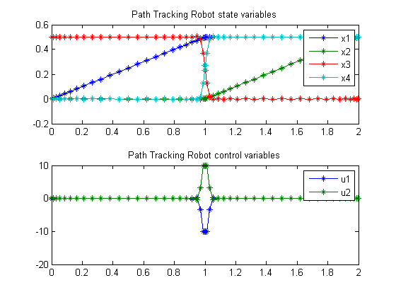
84.4  Plot result

subplot(2,1,1);
plot(t,x1,'*-',t,x2,'*-',t,x3,'*-',t,x4,'*-');
legend('x1','x2','x3','x4');
title('Path Tracking Robot state variables');

subplot(2,1,2);
plot(t,u1,'*-',t,u2,'*-');
legend('u1','u2');
title('Path Tracking Robot control variables');

« Previous « Start » Next »