« Previous « Start » Next »
56 Lee-Ramirez Bioreactor
Dynamic optimization of chemical and biochemical processes using restricted second-order information 2001, Eva Balsa-Canto, Julio R. Banga, Antonio A. Alonso Vassilios S. Vassiliadis
Case Study II: Lee-Ramirez bioreactor
56.1 Problem description
This problem considers the optimal control of a fed-batch reactor for induced foreign protein production by recombinant bacteria, as presented by Lee and Ramirez (1994) and considered afterwards by Tholudur and Ramirez (1997) and Carrasco and Banga (1998). The objective is to maximize the profitability of the process using the nutrient and the inducer feeding rates as the control variables. Three different values for the ratio of the cost of inducer to the value of the protein production (Q) were considered.
The mathematical formulation, following the modified parameter function set presented by Tholudur and Ramirez (1997) to increase the sensitivity to the controls, is as follows:
Find u1(t) and u2(t) over t in [t0 t_f] to maximize:
| J = x4(tf)*x1(tf) − Q* | ∫ | | u2 dt |
subject to:
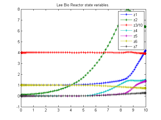
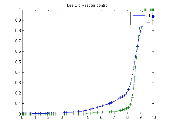
where the state variables are the reactor volume (x1), the cell density (x2), the nutrient concentration (x3), the foreign protein concentration (x4), the inducer concentration (x5), the inducer shock factor on cell growth rate (x6) and the inducer recovery factor on cell growth rate (x7). The two control variables are the glucose rate (u1) and the inducer feeding rate (u2). Q is the ratio of the cost of inducer to the value of the protein production, and the final time is considered fixed as t_f = 10 h. The model parameters were described by Lee and Ramirez (1994). The initial conditions are:
| x(t0) = [1 0.1 40 0 0 1 0]′ |
The following constraints on the control variables are considered:
Reference: [2]
56.2 Problem setup
toms t

for n=[20 35 55 85]
    p = tomPhase('p', t, 0, 10, n);
    setPhase(p);

    tomStates z1 z2 z3s z4 z5 z6 z7

    % Declaring u as "states" makes it possible to work with their
    % derivatives.
    tomStates u1 u2

    % Scale z3 by 40
    z3 = z3s*40;

    % Initial guess
    if n == 20
        x0 = {icollocate({z1 == 1; z2 == 0.1
            z3 == 40; z4 == 0; z5 == 0
            z6 == 1; z7 == 0})
            icollocate({u1==t/10; u2==t/10})};
    else
        x0 = {icollocate({z1 == z1opt
            z2 == z2opt; z3 == z3opt
            z4 == z4opt; z5 == z5opt
            z6 == z6opt; z7 == z7opt})
            icollocate({u1 == u1opt
            u2 == u2opt})};
    end

    % Box constraints
    cbox = {mcollocate({0 <= z1; 0 <= z2
        0 <= z3; 0 <= z4; 0 <= z5})
        0 <= collocate(u1) <= 1
        0 <= collocate(u2) <= 1};

    % Boundary constraints
    cbnd = initial({z1 == 1; z2 == 0.1
        z3 == 40; z4 == 0; z5 == 0
        z6 == 1; z7 == 0});

    % Various constants and expressions
    c1 = 100; c2 = 0.51; c3 = 4.0;
    Q  = 0;

    t1 = 14.35+z3+((z3).^2/111.5);
    t2 = 0.22+z5;
    t3 = z6+0.22./t2.*z7;

    g1 = z3./t1.*(z6+z7*0.22./t2);
    g2 = 0.233*z3./t1.*((0.0005+z5)./(0.022+z5));
    g3 = 0.09*z5./(0.034+z5);

    % ODEs and path constraints
    ceq = collocate({
        dot(z1) == u1+u2
        dot(z2) == g1.*z2-(u1+u2).*z2./z1
        dot(z3) == u1./z1.*c1-(u1+u2).*z3./z1-g1.*z2/c2
        dot(z4) == g2.*z2-(u1+u2).*z4./z1
        dot(z5) == u2*c3./z1-(u1+u2).*z5./z1
        dot(z6) == -g3.*z6
        dot(z7) == g3.*(1-z7)});

    % Objective
    J = -final(z1)*final(z4)+Q*integrate(u2);

    spenalty = 0.1/n; % penalty term to yield a smoother u.
    objective = J + spenalty*integrate(dot(u1)^2+dot(u2)^2);
56.3 Solve the problem
    options = struct;
    options.name = 'Lee Bio Reactor';
    solution = ezsolve(objective, {cbox, cbnd, ceq}, x0, options);

    % Optimal z, u for starting point
    z1opt = subs(z1, solution);
    z2opt = subs(z2, solution);
    z3opt = subs(z3, solution);
    z4opt = subs(z4, solution);
    z5opt = subs(z5, solution);
    z6opt = subs(z6, solution);
    z7opt = subs(z7, solution);
    u1opt = subs(u1, solution);
    u2opt = subs(u2, solution);
Problem type appears to be: qpcon
Starting numeric solver
===== * * * =================================================================== * * *
TOMLAB - Tomlab Optimization Inc. Development license  999001. Valid to 2011-02-05
=====================================================================================
Problem: ---  1: Lee Bio Reactor                f_k      -6.158549510890046500
                                       sum(|constr|)      0.000022911257182501
                              f(x_k) + sum(|constr|)     -6.158526599632864400
                                              f(x_0)      0.001000000000000008

Solver: snopt.  EXIT=0.  INFORM=1.
SNOPT 7.2-5 NLP code
Optimality conditions satisfied

FuncEv    1 ConstrEv  818 ConJacEv  818 Iter  628 MinorIter 3252
CPU time: 8.656250 sec. Elapsed time: 9.078000 sec.
Problem type appears to be: qpcon
Starting numeric solver
===== * * * =================================================================== * * *
TOMLAB - Tomlab Optimization Inc. Development license  999001. Valid to 2011-02-05
=====================================================================================
Problem: ---  1: Lee Bio Reactor                f_k      -6.149281872815334000
                                       sum(|constr|)      0.000001068521931031
                              f(x_k) + sum(|constr|)     -6.149280804293402600
                                              f(x_0)     -6.161206582021080200

Solver: snopt.  EXIT=0.  INFORM=1.
SNOPT 7.2-5 NLP code
Optimality conditions satisfied

FuncEv    1 ConstrEv  716 ConJacEv  716 Iter  639 MinorIter 2089
CPU time: 19.140625 sec. Elapsed time: 19.593000 sec.
Problem type appears to be: qpcon
Starting numeric solver
===== * * * =================================================================== * * *
TOMLAB - Tomlab Optimization Inc. Development license  999001. Valid to 2011-02-05
=====================================================================================
Problem: ---  1: Lee Bio Reactor                f_k      -6.148479057333524600
                                       sum(|constr|)      0.000000747224617591
                              f(x_k) + sum(|constr|)     -6.148478310108907300
                                              f(x_0)     -6.151340834042628100

Solver: snopt.  EXIT=0.  INFORM=1.
SNOPT 7.2-5 NLP code
Optimality conditions satisfied

FuncEv    1 ConstrEv  457 ConJacEv  457 Iter  400 MinorIter 1890
CPU time: 36.687500 sec. Elapsed time: 37.359000 sec.
Problem type appears to be: qpcon
Starting numeric solver
===== * * * =================================================================== * * *
TOMLAB - Tomlab Optimization Inc. Development license  999001. Valid to 2011-02-05
=====================================================================================
Problem: ---  1: Lee Bio Reactor                f_k      -6.149330683460276800
                                       sum(|constr|)      0.000000648177269734
                              f(x_k) + sum(|constr|)     -6.149330035283006700
                                              f(x_0)     -6.149452704290531800

Solver: snopt.  EXIT=0.  INFORM=1.
SNOPT 7.2-5 NLP code
Optimality conditions satisfied

FuncEv    1 ConstrEv  392 ConJacEv  392 Iter  341 MinorIter 2079
CPU time: 144.671875 sec. Elapsed time: 155.766000 sec.
end

t  = subs(collocate(t),solution);
z1 = subs(collocate(z1),solution);
z2 = subs(collocate(z2),solution);
z3 = subs(collocate(z3),solution);
z4 = subs(collocate(z4),solution);
z5 = subs(collocate(z5),solution);
z6 = subs(collocate(z6),solution);
z7 = subs(collocate(z7),solution);
u1 = subs(collocate(u1),solution);
u2 = subs(collocate(u2),solution);
56.4 Plot result
figure(1)
plot(t,z1,'*-',t,z2,'*-',t,z3/10,'*-',t,z4,'*-' ...
    ,t,z5,'*-',t,z6,'*-',t,z7,'*-');
legend('z1','z2','z3/10','z4','z5','z6','z7');
title('Lee Bio Reactor state variables.');

figure(2)
plot(t,u1,'+-',t,u2,'+-');
legend('u1','u2');
title('Lee Bio Reactor control');

disp('J = ');
disp(subs(J,solution));
J =
   -6.1510
« Previous « Start » Next »
