« Previous « Start » Next »

52  Initial Value Problem

On some linear-quadratic optimal control problems for descriptor systems. Galina Kurina, Department of Mathematics, Stockholm University, Sweden.

2.5 Necessary control optimality conditions is not valid in general case.

52.1  Problem Description

Find u over t in [0; 1 ] to minimize:

J =

1 2

*x12(0.5) +

1 2

*x12(1) +

1 2

*

∫

1 0

u2 dt

subject to:

dx1 dt

= x3+u

dx2 dt

= x2−x3+u

x2 = 0

x(t0) = [5  0  NaN]

Reference: [21]

52.2  Problem setup

toms t1
p1 = tomPhase('p1', t1, 0, 0.5, 20);
setPhase(p1);

tomStates x1p1 x2p1
tomControls x3p1 up1

% Initial guess
x01 = {icollocate({x1p1 == 0; x2p1 == 0})
    collocate({x3p1 == 0; up1 == 0})};

% Boundary constraints
cbnd1 = initial({x1p1 == 5; x2p1 == 0});

% ODEs and path constraints
ceq1 = collocate({
    dot(x1p1) == x3p1+up1
    dot(x2p1) == x2p1-x3p1+up1
    dot(x2p1) == 0});

% Objective
objective1 = 0.5*final(x1p1)^2+0.5*integrate(up1.^2);

toms t2
p2 = tomPhase('p2', t2, 0.5, 0.5, 20);
setPhase(p2);

tomStates x1p2 x2p2
tomControls x3p2 up2

% Initial guess
x02 = {icollocate({x1p2 == 0; x2p2 == 0})
    collocate({x3p2 == 0; up2 == 0})};

% ODEs and path constraints
ceq2 = collocate({
    dot(x1p2) == x3p2+up2
    dot(x2p2) == x2p2-x3p2+up2
    dot(x2p2) == 0});

% Objective
objective2 = 0.5*final(x1p2)^2+0.5*integrate(up2.^2);
objective = objective1 + objective2;

% Link phase
link = {final(p1,x1p1) == initial(p2,x1p2)
    final(p1,x2p1) == initial(p2,x2p2)
    final(p1,x3p1) == initial(p2,x3p2)};

52.3  Solve the problem

options = struct;
options.name = 'Initial Value Problem';
options.solver = 'snopt';
constr = {cbnd1, ceq1, ceq2, link};
solution = ezsolve(objective, constr, {x01, x02}, options);

Problem type appears to be: qp
Starting numeric solver
===== * * * =================================================================== * * *
TOMLAB - Tomlab Optimization Inc. Development license  999001. Valid to 2011-02-05
=====================================================================================
Problem:  1: Initial Value Problem              f_k       4.550747663987713100
                                       sum(|constr|)      0.000000000451074017
                              f(x_k) + sum(|constr|)      4.550747664438787000
                                              f(x_0)     12.499999999999893000

Solver: snopt.  EXIT=0.  INFORM=1.
SNOPT 7.2-5 NLP code
Optimality conditions satisfied

FuncEv    1 Iter   23 MinorIter  142
CPU time: 0.031250 sec. Elapsed time: 0.031000 sec.

52.4  Plot result

subplot(3,1,1)
t  = [subs(collocate(p1,t1),solution);subs(collocate(p2,t2),solution)];
x1 = [subs(collocate(p1,x1p1),solution);subs(collocate(p2,x1p2),solution)];
x2 = [subs(collocate(p1,x2p1),solution);subs(collocate(p2,x2p2),solution)];
u  = [subs(collocate(p1,up1),solution);subs(collocate(p2,up2),solution)];

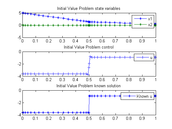
plot(t,x1,'*-',t,x2,'*-');
legend('x1','x2');
title('Initial Value Problem state variables');

subplot(3,1,2)
plot(t,u,'+-');
legend('u');
title('Initial Value Problem control');

subplot(3,1,3)
plot(t,-8/11*5*(t<0.5)-2/11*5*(t>=0.5),'*-');
legend('Known u');
title('Initial Value Problem known solution');

« Previous « Start » Next »